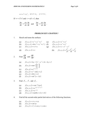
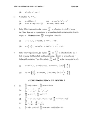
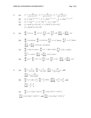
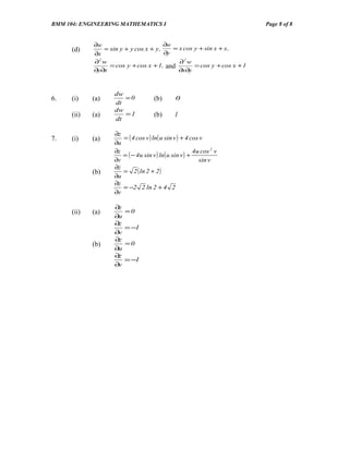
SlideShare a Scribd company logo
BMM 104: ENGINEERING MATHEMATICS I                                                       Page 1 of 8


                                CHAPTER 5: PARTIAL DERIVATIVES

Functions of n Independent Variables

Suppose D is a set of n-tuples of real numbers ( x1 , x 2 ,..., x n ) . A real valued function f
on D is a rule that assigns a unique (single) real number

                 w = f ( x1 , x 2 ,..., x n )
to each element in D. The set D is the function’s domain. The set of w-values taken on
by f is the function’s range. The symbol w is the dependent variable of f, and f is said to
be a function of the n independent variables x1 to x n . We also call the x j ' s the
function’s input variables and call w the function’s output variable.

Level Curve, Graph, surface of Functions of Two Variables

The set of points in the plane where a function f ( x , y ) has a constant value f ( x , y ) = c
is called a level curve of f. The set of all points ( x , y , f ( x , y ) ) in space, for ( x , y ) in
the domain of f, is called the graph of f. The graph of f is also called the surface
 z = f ( x , y) .

Functions of Three Variables

The set of points ( x , y , z ) in space where a function of three independent variables has a
constant value f ( x , y , z ) = c is called a level surface of f.

Example: Attend lecture.

Partial Derivatives of a Function of Two Variables

Definition:      Partial Derivative with Respect to x

The partial derivative of f ( x , y ) with respect to x at the point ( x0 , y 0 ) is

                 ∂f                         f ( x0 + h , y 0 ) − f ( x0 , y 0 )
                                    = lim                                       ,
                 ∂x   ( x0 , y0 )
                                      h→0                   h
provided the limit exists.


Definition:      Partial Derivative with Respect to y
BMM 104: ENGINEERING MATHEMATICS I                                                                                        Page 2 of 8


The partial derivative of f ( x , y ) with respect to y at the point ( x0 , y0 ) is

                    ∂f                     d                                      f ( x0 , y 0 + h ) − f ( x0 , y 0 )
                                       =      f ( x0 , y )             = lim                                          ,
                    ∂y   ( x0 , y0 )       dy                 y = y0        h→0                   h
provided the limit exists.

Example:

                                           ∂f     ∂f
1.       Find the values of                   and ∂ at the point ( 4 ,− ) if
                                                                       5
                                           ∂x      y
 f ( x , y ) = x 2 + 3 xy + y − 1 .
                   ∂ f
2.           Find         if f ( x , y ) = y sin xy .
                    ∂ x
                                                                       2y
3.       Find f x and f y if f ( x , y ) = y + cos x .


Functions of More Than Two Variables

Example:

                                                             ∂f   ∂f    ∂f
1.       Let f ( x , y , z ) = xy 2 z 3 . Find                  , ∂ and    at (1,− ,− ) .
                                                                                  2 1
                                                             ∂x    y    ∂z
                                             y
2.       Let g ( x , y , z ) = x 2 e z . Find g x , g y and g z .


Second-Order Partial Derivatives

When we differentiate a function f ( x , y ) twice, we produce its second-order
       derivatives.
These derivatives are usually denoted by

∂2 f                                                         f xx
         “ d squared fdx squared “ or                                   “f sub xx “
∂x 2

∂2 f
         “ d squared fdy squared “ or                        f yy       “f sub yy “
∂ 2
 y

∂2 f                                                         f xx
         “ d squared fdx squared “ or                                   “f sub xx “
∂x 2

 ∂ f
  2

                   “ d squared fdxdy squared “ or                                      f yx     “f sub yx “
 ∂∂
  x y
BMM 104: ENGINEERING MATHEMATICS I                                                                               Page 3 of 8


∂ f
 2

                  “ d squared fdydx squared “ or                                       f xy        “f sub xy “
∂∂
 y x

The defining equations are

                   ∂2 f   ∂  ∂f                          ∂2 f   ∂ ∂ 
                                                                       f
                        =        ,                            =    
                                                                     ∂ 
                   ∂x 2
                          ∂x  ∂x                         ∂∂
                                                            x y   ∂  y
                                                                   x     
and so on. Notice the order in which the derivatives are taken:

         ∂ f
          2

                                             Differentiate first with respect to y, then with respect to x.
         ∂∂
          x y

         f yx = ( f y ) x      Means the same thing.

Example:

                                                ∂2 f    ∂ f
                                                          2
                                                                ∂ f        ∂ f
                                                                             2                      2

1.      Let f ( x , y ) = x 3 y 2 − x 4 y 6 . Find    ,       ,        and       .
                                                 ∂x 2 ∂ ∂ ∂
                                                          y x     y2       ∂∂x y
                                               ∂2 f   ∂ f
                                                        2
                                                              ∂2 f        ∂ f
                                                                           2

2.      If f ( x , y ) = x cos y + ye x , find      ,       ,        and       .
                                               ∂x 2 ∂ ∂ ∂
                                                        y x     y2       ∂∂x y


The Chain Rule

Chain Rule for Functions of Two Independent Variables

If w = f ( x , y ) has continuous partial derivatives f x and f y and if x = x( t ) , y = y ( t )
        are
differentiable functions of t, then the compose w = f ( x( t ) , y ( t ) ) is a differentiable
function of t and

                   df
                      = f x ( x ( t ) , y ( t ) ) • x ' ( t ) + f y ( x( t ) , y ( t ) ) • y ' ( t ) ,
                   dt

or
                   dw   ∂f dx ∂f dy
                      =       +       .
                   dt   ∂x dt   ∂y dt

Example:

Use the chain rule to find the derivative of w = xy , with respect to t along the path
BMM 104: ENGINEERING MATHEMATICS I                                                              Page 4 of 8


                                                             π
x = cos t , y = sin t . What is the derivative’s value at t = ?
                                                                       2

Chain Rule for Functions of Three Independent Variables

If w = f ( x , y , z ) is differentiable and x, y and z are differentiable functions of t, then w
        is
a differentiable function of t and

                   dw   ∂f dx ∂f dy ∂f dz
                      =       +       +       .
                   dt   ∂x dt   ∂y dt   ∂z dt

Example:

       dw
Find      if w = xy + z ,      x = cos t ,   y = sin t ,   z =t.
       dt

Chain Rule for Two Independent Variables and Three Intermediate Variables

Suppose that w = f ( x , y , z ) , x = g ( r , s ) , y = h( r , s ) , and z = k ( r , s ) . If all four
        functions
are differentiable, then w has partial derivatives with respect to r and s, given by the
formulas

                   ∂w   ∂ ∂
                         w x ∂ ∂w y   ∂ ∂
                                       w z
                      =      +      +
                   ∂r   ∂ ∂
                         x r   ∂ ∂
                                y r   ∂ ∂
                                       z r

                   ∂w   ∂ ∂
                         w x ∂ ∂w y   ∂ ∂
                                       w z
                      =      +      +
                   ∂s   ∂ ∂
                         x s   ∂ ∂
                                y s   ∂ ∂
                                       z s

Example:

           ∂w     ∂w
Express       and               in terms of r and s is
           ∂r     ∂s

                                    r
         w = x +2y + z2, x =          , y = r 2 + ln s , z = 2 r .
                                    s

If w = f ( x , y ) , x = g ( r , s ) , and y = h( r , s ) , then

          ∂w   ∂ ∂
                w x   ∂ ∂
                       w y                                         ∂w   ∂ ∂
                                                                         w x   ∂ ∂
                                                                                w y
             =      +                                  and            =      +
          ∂r   ∂ ∂
                x r   ∂ ∂
                       y r                                         ∂s   ∂ ∂
                                                                         x s   ∂ ∂
                                                                                y s
Example:

           ∂w     ∂w
Express       and    in terms of r and s if
           ∂r     ∂s
BMM 104: ENGINEERING MATHEMATICS I                                                                   Page 5 of 8


         w = x2 + y2 ,     x= r− s,                  y =r+s.

If w = f ( x ) and x = g ( r , s ) , then

         ∂w   dw ∂x                     ∂w   dw ∂x
            =       and                    =       .
         ∂r   dx ∂r                     ∂s   dx ∂s


                                     PROBLEM SET: CHAPTER 5

1.      Sketch and name the surfaces

        (a)       f ( x, y , z ) = x 2 + y 2 + z 2        (e)        f ( x, y, z ) = x 2 + y 2
        (b)       f ( x , y , z ) = ln( x 2 + y 2 + z 2 ) (f)        f ( x, y, z ) = y 2 + z 2
        (c)       f ( x, y , z ) = x + z                  (g)        f ( x, y, z ) = z − x 2 − y 2
                                                                                                 x2 y2 z2
        (d)       f ( x, y, z ) = z                                  (h)      f ( x, y , z ) =     +   +
                                                                                                 25 16   9

               ∂f     ∂f
2.      Find      and ∂ .
               ∂x      y

        (a)       f ( x , y ) = 5 xy − 7 x 2 − y 2 + 3 x − 6 y + 2
                                           y
        (b)       f ( x , y ) = tan −1  
                                           x
        (c)       f ( x, y) = e    ( x + y +1)

        (d)       f ( x , y ) = e −x sin( x + y )
        (e)       f ( x , y ) = ln( x + y )
        (f)       f ( x , y ) = sin 2 ( x − 3 y )

3.      Find f x , f y and f z .

        (a)       f ( x , y , z ) = sin −1 ( xyz )
                  f ( x , y , z ) = e −( x                    )
                                             2
                                                 + y 2 +z 2
        (b)
        (c)       f ( x , y , z ) = e −xyz
        (d)       f ( x , y , z ) = tanh( x + 2 y + 3 z )

4.      Find all the second-order partial derivatives of the following functions.

        (a)       f ( x , y ) = x + y + xy
        (b)       f ( x , y ) = sin xy
        (c)       f ( x , y ) = x 2 y + cos y + y sin x
BMM 104: ENGINEERING MATHEMATICS I                                                                      Page 6 of 8


      (d)      f ( x , y ) = xe y + y + 1

5.    Verify that w xy = w yx .

      (a)     w = ln( 2 x + 3 y )                       (c)      w = xy 2 + x 2 y 3 + x 3 y 4
      (b)     w = e x + x ln y + y ln x (d)              w = x sin y + y sin x + xy

                                                            dw
6.    In the following questions, (a) express                  as a function of t, both by using
                                                            dt
      the Chain Rule and by expressing w in terms of t and differentiating directly with
                                              dw
      respect to t. The (b) evaluate             at the given value of t.
                                              dt

      (i)     w = x2 + y2 ,        x = cos t ,      y = sin t ;      t=π .

                    x y                                                     1
      (ii)    w=     + ,         x = cos 2 t ,      y = sin 2 t ,     z=          t =3.
                    z z                                                     t

                                                            ∂z     ∂z
7.    In the following questions, (a) express                  and    as a functions of u and v
                                                            ∂u     ∂v
      both by using the Chain Rule and by expressing z directly in terms of u and v
                                                              ∂z     ∂z
      before differentiating. Then (b) evaluate                  and    at the given point (u , v ) .
                                                              ∂u     ∂v


      (i)     z = 4 e x ln y ,      x = ln( u cos v ) ,       y = u sin v ;      ( u ,v ) =  2 , π 
                                                                                                   
                                                                                                4


      (ii)
                         x
              z = tan −1   ,
                         y          x = u cos v ,       y = u sin v ;       ( u ,v ) = 1.3 , π 
                                                                                                 
                                                                                              6


                    ANSWERS FOR PROBLEM SET: CHAPTER 5

              ∂f                       ∂f
2.    (a)        = 5 y − 14 x + 3 ,        = 5 x − 2 y −6
              ∂x                       ∂y
              ∂f           y        ∂f          x
      (b)        =− 2             ,     = 2
              ∂x     x + y 2 ∂y           x + y2
              ∂f                   ∂f
      (c)        = e ( x +y +1) ,      = e ( x +y +1 )
              ∂x                   ∂y
              ∂f                                             ∂f
      (d)        = −e −x sin( x + y ) + e −x cos ( x + y ) ,    = e −x cos ( x + y )
              ∂x                                             ∂y
              ∂f     1    ∂f    1
      (e)        =      ,    =
              ∂x   x + y ∂y    x+y
              ∂f                                     ∂f
      (f)        = 2 sin( x − 3 y ) cos( x − 3 y ) ,    = −6 sin( x − 3 y ) cos( x − 3 y )
              ∂x                                     ∂x
BMM 104: ENGINEERING MATHEMATICS I                                                                                Page 7 of 8


                            yz                                xz                                   xy
3.    (a)     fx =                            , fy =                          , fz =
                       1−x y z2       2   2
                                                          1−x y z
                                                                2   2   2
                                                                                              1 − x2 y2 z2
              f x = −2 xe −( x                     ) , f = −2 ye −( x                        f z = −2 ze − ( x + y + z )
      (b)
                                  2
                                      + y 2 +z 2                        2
                                                                            + y 2 +z 2   ) ,                  2   2   2
                                                        y

      (c)     f x = −yze −xyz , f y = −xze −xyz , f z = −xye − xyz
      (d)     f x = sec h 2 ( x + 2 y + 3 z ) , f y = 2 sec h 2 ( x + 2 y + 3 z ) ,
              f z = 3 sec h 2 ( x + 2 y + 3 z )

              ∂f          ∂f                   ∂2 f
                             =1 + x , ∂ f = 0,
                                       2
                                                         ∂2 f   ∂2 f
4.    (a)        = 1 + y,                           = 0,      =      =1
              ∂x          ∂y          ∂x 2     ∂y 2      ∂∂
                                                          y x   ∂∂
                                                                 x y


              ∂f              ∂f                                   ∂2 f
                                 = x cos xy , ∂ f = − y 2 sin xy ,
                                               2
      (b)        = y cos xy ,                                           = −x 2 sin xy ,
              ∂x              ∂y              ∂x 2                 ∂y 2
              ∂2 f   ∂2 f
                   =      = cos xy − xy sin xy
              ∂y∂x   ∂x∂y
              ∂f                     ∂f
                                        = x 2 − sin y + sin x , ∂ f = 2 y − y sin x ,
                                                                 2
      (c)         = 2 xy + y cos x ,
              ∂x                     ∂y                         ∂x 2
              ∂ f
               2
                               ∂2 f     ∂2 f
                   = −cos y ,         =       = 2 x + cos x
              ∂y 2
                               ∂y∂x     ∂x∂y
              ∂f     ∂f                        ∂2 f
                        = xe y + 1 , ∂ f = 0 ,
                                      2
                                                             ∂2 f   ∂2 f
      (d)        =ey                                = xe y ,      =      =e y
              ∂x     ∂y              ∂x 2      ∂y 2
                                                             ∂∂
                                                              y x   ∂∂
                                                                     x y


              ∂w       2      ∂w       3      ∂2 w       −6
5.    (a)        =          ,    =          ,      =              , and
              ∂x   2 x + 3 y ∂y    2 x + 3 y ∂y∂x    (2x + 3 y) 2
              ∂2 w       −6
                   =
              ∂x∂y ( 2 x + 3 y ) 2
              ∂w               y ∂w  x         ∂2 w  1 1
      (b)        = e x + ln y + ,   = + ln x ,      = + , and
              ∂x               x ∂y  y         ∂∂
                                                y x  y x
              ∂2w 1 1
                  = +
              ∂x∂y y x

              ∂w                              ∂w
      (c)        = y 2 + 2 xy 3 + 3 x 2 y 4 ,    = 2 xy + 3 x 2 y 2 + 4 x 3 y 3 ,
              ∂x                              ∂y
      ∂2 w                                   ∂2 w
           = 2 y + 6 xy 2 + 12 x 2 y 3 , and      = 2 y + 6 xy 2 + 12 x 2 y 3
      ∂y∂x                                   ∂x∂y
BMM 104: ENGINEERING MATHEMATICS I                                        Page 8 of 8


             ∂w                         ∂w
      (d)       = sin y + y cos x + y ,    = x cos y + sin x + x ,
             ∂x                         ∂y
             ∂2 w                          ∂2 w
                  = cos y + cos x + 1, and      = cos y + cos x + 1
             ∂y∂x                          ∂x∂y


                     dw
6.    (i)    (a)        =0              (b)       0
                     dt
                     dw
      (ii)   (a)        =1              (b)       1
                     dt

                     ∂z
7.    (i)    (a)          = ( 4 cos v ) ln( u sin v ) + 4 cos v
                     ∂u
                     ∂z                                      4u cos 2 v
                          = ( − 4u sin v ) ln( u sin v ) +
                     ∂v                                        sin v
                     ∂z
             (b)          = 2 ( ln 2 + 2 )
                     ∂u
                     ∂z
                          = −2 2 ln 2 + 4 2
                     ∂v

                     ∂z
      (ii)   (a)          =0
                     ∂u
                     ∂z
                          = −1
                     ∂v
                     ∂z
             (b)          =0
                     ∂u
                     ∂z
                          = −1
                     ∂v

More Related Content

What's hot

Partial Differentiation
Partial DifferentiationPartial Differentiation
Partial Differentiation
Deep Dalsania
 
Chapter 16 2
Chapter 16 2Chapter 16 2
Chapter 16 2
EasyStudy3
 
Multiple ppt
Multiple pptMultiple ppt
Multiple ppt
Manish Mor
 
1st order differential equations
1st order differential equations1st order differential equations
1st order differential equations
Nisarg Amin
 
Differential Equations
Differential EquationsDifferential Equations
Differential Equations
KrupaSuthar3
 
Transformada de fourier (mate 4)
Transformada de fourier (mate 4)Transformada de fourier (mate 4)
Transformada de fourier (mate 4)
YeismarAraque
 
Continuity and differentiability
Continuity and differentiability Continuity and differentiability
Continuity and differentiability
Seyid Kadher
 
Techniques of Integration ppt.ppt
Techniques of Integration ppt.pptTechniques of Integration ppt.ppt
Techniques of Integration ppt.ppt
JaysonFabela1
 
What is analytic functions
What is analytic functionsWhat is analytic functions
What is analytic functions
Tarun Gehlot
 
Dobule and triple integral
Dobule and triple integralDobule and triple integral
Dobule and triple integral
sonendra Gupta
 
Limits and continuity
Limits and continuityLimits and continuity
Limits and continuity
Digvijaysinh Gohil
 
Complex function
Complex functionComplex function
Complex function
Dr. Nirav Vyas
 
First order linear differential equation
First order linear differential equationFirst order linear differential equation
First order linear differential equation
Nofal Umair
 
Curve sketching
Curve sketchingCurve sketching
Curve sketching
Rnold Wilson
 
4.1 inverse functions
4.1 inverse functions4.1 inverse functions
4.1 inverse functions
math260
 
30 surface integrals
30 surface integrals30 surface integrals
30 surface integrals
math267
 
DIFFERENTIAL EQUATIONS
DIFFERENTIAL EQUATIONSDIFFERENTIAL EQUATIONS
DIFFERENTIAL EQUATIONS
Urmila Bhardwaj
 
Integrales
IntegralesIntegrales
Mean Value Theorem | Mathematics
Mean Value Theorem | MathematicsMean Value Theorem | Mathematics
Mean Value Theorem | Mathematics
askIITians - Creating Engineers & Doctors
 
Functions and its Applications in Mathematics
Functions and its Applications in MathematicsFunctions and its Applications in Mathematics
Functions and its Applications in Mathematics
Amit Amola
 

What's hot (20)

Partial Differentiation
Partial DifferentiationPartial Differentiation
Partial Differentiation
 
Chapter 16 2
Chapter 16 2Chapter 16 2
Chapter 16 2
 
Multiple ppt
Multiple pptMultiple ppt
Multiple ppt
 
1st order differential equations
1st order differential equations1st order differential equations
1st order differential equations
 
Differential Equations
Differential EquationsDifferential Equations
Differential Equations
 
Transformada de fourier (mate 4)
Transformada de fourier (mate 4)Transformada de fourier (mate 4)
Transformada de fourier (mate 4)
 
Continuity and differentiability
Continuity and differentiability Continuity and differentiability
Continuity and differentiability
 
Techniques of Integration ppt.ppt
Techniques of Integration ppt.pptTechniques of Integration ppt.ppt
Techniques of Integration ppt.ppt
 
What is analytic functions
What is analytic functionsWhat is analytic functions
What is analytic functions
 
Dobule and triple integral
Dobule and triple integralDobule and triple integral
Dobule and triple integral
 
Limits and continuity
Limits and continuityLimits and continuity
Limits and continuity
 
Complex function
Complex functionComplex function
Complex function
 
First order linear differential equation
First order linear differential equationFirst order linear differential equation
First order linear differential equation
 
Curve sketching
Curve sketchingCurve sketching
Curve sketching
 
4.1 inverse functions
4.1 inverse functions4.1 inverse functions
4.1 inverse functions
 
30 surface integrals
30 surface integrals30 surface integrals
30 surface integrals
 
DIFFERENTIAL EQUATIONS
DIFFERENTIAL EQUATIONSDIFFERENTIAL EQUATIONS
DIFFERENTIAL EQUATIONS
 
Integrales
IntegralesIntegrales
Integrales
 
Mean Value Theorem | Mathematics
Mean Value Theorem | MathematicsMean Value Theorem | Mathematics
Mean Value Theorem | Mathematics
 
Functions and its Applications in Mathematics
Functions and its Applications in MathematicsFunctions and its Applications in Mathematics
Functions and its Applications in Mathematics
 

Similar to Chapter 5(partial differentiation)

Bernheim calculusfinal
Bernheim calculusfinalBernheim calculusfinal
Bernheim calculusfinal
rahulrasa
 
Lesson 8: Basic Differentation Rules (slides)
Lesson 8: Basic Differentation Rules (slides)Lesson 8: Basic Differentation Rules (slides)
Lesson 8: Basic Differentation Rules (slides)
Mel Anthony Pepito
 
Lesson 8: Basic Differentation Rules (slides)
Lesson 8: Basic Differentation Rules (slides)Lesson 8: Basic Differentation Rules (slides)
Lesson 8: Basic Differentation Rules (slides)
Matthew Leingang
 
584 fundamental theorem of calculus
584 fundamental theorem of calculus584 fundamental theorem of calculus
584 fundamental theorem of calculus
goldenratio618
 
Chapter 16
Chapter 16Chapter 16
Chapter 16
ramiz100111
 
Lattices and codes
Lattices and codesLattices and codes
Lattices and codes
Springer
 
Partial Derivatives.pdf
Partial Derivatives.pdfPartial Derivatives.pdf
Partial Derivatives.pdf
NanavathAkkashChandr
 
Lesson 8: Basic Differentiation Rules
Lesson 8: Basic Differentiation RulesLesson 8: Basic Differentiation Rules
Lesson 8: Basic Differentiation Rules
Matthew Leingang
 
test
testtest
Chapter 3
Chapter 3Chapter 3
Chapter 3
aabdel96
 
Quantum modes - Ion Cotaescu
Quantum modes - Ion CotaescuQuantum modes - Ion Cotaescu
Quantum modes - Ion Cotaescu
SEENET-MTP
 
Complex varible
Complex varibleComplex varible
Complex varible
Naveen Sihag
 
Complex varible
Complex varibleComplex varible
Complex varible
Naveen Sihag
 
Difrentiation
DifrentiationDifrentiation
Difrentiation
lecturer
 
[Vvedensky d.] group_theory,_problems_and_solution(book_fi.org)
[Vvedensky d.] group_theory,_problems_and_solution(book_fi.org)[Vvedensky d.] group_theory,_problems_and_solution(book_fi.org)
[Vvedensky d.] group_theory,_problems_and_solution(book_fi.org)
Dabe Milli
 
Ex algebra (5)
Ex algebra  (5)Ex algebra  (5)
Ex algebra (5)
Andrei Bastos
 
subdiff_prox.pdf
subdiff_prox.pdfsubdiff_prox.pdf
subdiff_prox.pdf
diehardgamer1
 
Lesson 8: Basic Differentiation Rules
Lesson 8: Basic Differentiation RulesLesson 8: Basic Differentiation Rules
Lesson 8: Basic Differentiation Rules
Matthew Leingang
 
Limits
LimitsLimits
Lesson 8: Basic Differentiation Rules
Lesson 8: Basic Differentiation RulesLesson 8: Basic Differentiation Rules
Lesson 8: Basic Differentiation Rules
Matthew Leingang
 

Similar to Chapter 5(partial differentiation) (20)

Bernheim calculusfinal
Bernheim calculusfinalBernheim calculusfinal
Bernheim calculusfinal
 
Lesson 8: Basic Differentation Rules (slides)
Lesson 8: Basic Differentation Rules (slides)Lesson 8: Basic Differentation Rules (slides)
Lesson 8: Basic Differentation Rules (slides)
 
Lesson 8: Basic Differentation Rules (slides)
Lesson 8: Basic Differentation Rules (slides)Lesson 8: Basic Differentation Rules (slides)
Lesson 8: Basic Differentation Rules (slides)
 
584 fundamental theorem of calculus
584 fundamental theorem of calculus584 fundamental theorem of calculus
584 fundamental theorem of calculus
 
Chapter 16
Chapter 16Chapter 16
Chapter 16
 
Lattices and codes
Lattices and codesLattices and codes
Lattices and codes
 
Partial Derivatives.pdf
Partial Derivatives.pdfPartial Derivatives.pdf
Partial Derivatives.pdf
 
Lesson 8: Basic Differentiation Rules
Lesson 8: Basic Differentiation RulesLesson 8: Basic Differentiation Rules
Lesson 8: Basic Differentiation Rules
 
test
testtest
test
 
Chapter 3
Chapter 3Chapter 3
Chapter 3
 
Quantum modes - Ion Cotaescu
Quantum modes - Ion CotaescuQuantum modes - Ion Cotaescu
Quantum modes - Ion Cotaescu
 
Complex varible
Complex varibleComplex varible
Complex varible
 
Complex varible
Complex varibleComplex varible
Complex varible
 
Difrentiation
DifrentiationDifrentiation
Difrentiation
 
[Vvedensky d.] group_theory,_problems_and_solution(book_fi.org)
[Vvedensky d.] group_theory,_problems_and_solution(book_fi.org)[Vvedensky d.] group_theory,_problems_and_solution(book_fi.org)
[Vvedensky d.] group_theory,_problems_and_solution(book_fi.org)
 
Ex algebra (5)
Ex algebra  (5)Ex algebra  (5)
Ex algebra (5)
 
subdiff_prox.pdf
subdiff_prox.pdfsubdiff_prox.pdf
subdiff_prox.pdf
 
Lesson 8: Basic Differentiation Rules
Lesson 8: Basic Differentiation RulesLesson 8: Basic Differentiation Rules
Lesson 8: Basic Differentiation Rules
 
Limits
LimitsLimits
Limits
 
Lesson 8: Basic Differentiation Rules
Lesson 8: Basic Differentiation RulesLesson 8: Basic Differentiation Rules
Lesson 8: Basic Differentiation Rules
 

Chapter 5(partial differentiation)

  • 1. BMM 104: ENGINEERING MATHEMATICS I Page 1 of 8 CHAPTER 5: PARTIAL DERIVATIVES Functions of n Independent Variables Suppose D is a set of n-tuples of real numbers ( x1 , x 2 ,..., x n ) . A real valued function f on D is a rule that assigns a unique (single) real number w = f ( x1 , x 2 ,..., x n ) to each element in D. The set D is the function’s domain. The set of w-values taken on by f is the function’s range. The symbol w is the dependent variable of f, and f is said to be a function of the n independent variables x1 to x n . We also call the x j ' s the function’s input variables and call w the function’s output variable. Level Curve, Graph, surface of Functions of Two Variables The set of points in the plane where a function f ( x , y ) has a constant value f ( x , y ) = c is called a level curve of f. The set of all points ( x , y , f ( x , y ) ) in space, for ( x , y ) in the domain of f, is called the graph of f. The graph of f is also called the surface z = f ( x , y) . Functions of Three Variables The set of points ( x , y , z ) in space where a function of three independent variables has a constant value f ( x , y , z ) = c is called a level surface of f. Example: Attend lecture. Partial Derivatives of a Function of Two Variables Definition: Partial Derivative with Respect to x The partial derivative of f ( x , y ) with respect to x at the point ( x0 , y 0 ) is ∂f f ( x0 + h , y 0 ) − f ( x0 , y 0 ) = lim , ∂x ( x0 , y0 ) h→0 h provided the limit exists. Definition: Partial Derivative with Respect to y
  • 2. BMM 104: ENGINEERING MATHEMATICS I Page 2 of 8 The partial derivative of f ( x , y ) with respect to y at the point ( x0 , y0 ) is ∂f d f ( x0 , y 0 + h ) − f ( x0 , y 0 ) = f ( x0 , y ) = lim , ∂y ( x0 , y0 ) dy y = y0 h→0 h provided the limit exists. Example: ∂f ∂f 1. Find the values of and ∂ at the point ( 4 ,− ) if 5 ∂x y f ( x , y ) = x 2 + 3 xy + y − 1 . ∂ f 2. Find if f ( x , y ) = y sin xy . ∂ x 2y 3. Find f x and f y if f ( x , y ) = y + cos x . Functions of More Than Two Variables Example: ∂f ∂f ∂f 1. Let f ( x , y , z ) = xy 2 z 3 . Find , ∂ and at (1,− ,− ) . 2 1 ∂x y ∂z y 2. Let g ( x , y , z ) = x 2 e z . Find g x , g y and g z . Second-Order Partial Derivatives When we differentiate a function f ( x , y ) twice, we produce its second-order derivatives. These derivatives are usually denoted by ∂2 f f xx “ d squared fdx squared “ or “f sub xx “ ∂x 2 ∂2 f “ d squared fdy squared “ or f yy “f sub yy “ ∂ 2 y ∂2 f f xx “ d squared fdx squared “ or “f sub xx “ ∂x 2 ∂ f 2 “ d squared fdxdy squared “ or f yx “f sub yx “ ∂∂ x y
  • 3. BMM 104: ENGINEERING MATHEMATICS I Page 3 of 8 ∂ f 2 “ d squared fdydx squared “ or f xy “f sub xy “ ∂∂ y x The defining equations are ∂2 f ∂  ∂f  ∂2 f ∂ ∂  f =  , =  ∂  ∂x 2 ∂x  ∂x  ∂∂ x y ∂  y x  and so on. Notice the order in which the derivatives are taken: ∂ f 2 Differentiate first with respect to y, then with respect to x. ∂∂ x y f yx = ( f y ) x Means the same thing. Example: ∂2 f ∂ f 2 ∂ f ∂ f 2 2 1. Let f ( x , y ) = x 3 y 2 − x 4 y 6 . Find , , and . ∂x 2 ∂ ∂ ∂ y x y2 ∂∂x y ∂2 f ∂ f 2 ∂2 f ∂ f 2 2. If f ( x , y ) = x cos y + ye x , find , , and . ∂x 2 ∂ ∂ ∂ y x y2 ∂∂x y The Chain Rule Chain Rule for Functions of Two Independent Variables If w = f ( x , y ) has continuous partial derivatives f x and f y and if x = x( t ) , y = y ( t ) are differentiable functions of t, then the compose w = f ( x( t ) , y ( t ) ) is a differentiable function of t and df = f x ( x ( t ) , y ( t ) ) • x ' ( t ) + f y ( x( t ) , y ( t ) ) • y ' ( t ) , dt or dw ∂f dx ∂f dy = + . dt ∂x dt ∂y dt Example: Use the chain rule to find the derivative of w = xy , with respect to t along the path
  • 4. BMM 104: ENGINEERING MATHEMATICS I Page 4 of 8 π x = cos t , y = sin t . What is the derivative’s value at t = ? 2 Chain Rule for Functions of Three Independent Variables If w = f ( x , y , z ) is differentiable and x, y and z are differentiable functions of t, then w is a differentiable function of t and dw ∂f dx ∂f dy ∂f dz = + + . dt ∂x dt ∂y dt ∂z dt Example: dw Find if w = xy + z , x = cos t , y = sin t , z =t. dt Chain Rule for Two Independent Variables and Three Intermediate Variables Suppose that w = f ( x , y , z ) , x = g ( r , s ) , y = h( r , s ) , and z = k ( r , s ) . If all four functions are differentiable, then w has partial derivatives with respect to r and s, given by the formulas ∂w ∂ ∂ w x ∂ ∂w y ∂ ∂ w z = + + ∂r ∂ ∂ x r ∂ ∂ y r ∂ ∂ z r ∂w ∂ ∂ w x ∂ ∂w y ∂ ∂ w z = + + ∂s ∂ ∂ x s ∂ ∂ y s ∂ ∂ z s Example: ∂w ∂w Express and in terms of r and s is ∂r ∂s r w = x +2y + z2, x = , y = r 2 + ln s , z = 2 r . s If w = f ( x , y ) , x = g ( r , s ) , and y = h( r , s ) , then ∂w ∂ ∂ w x ∂ ∂ w y ∂w ∂ ∂ w x ∂ ∂ w y = + and = + ∂r ∂ ∂ x r ∂ ∂ y r ∂s ∂ ∂ x s ∂ ∂ y s Example: ∂w ∂w Express and in terms of r and s if ∂r ∂s
  • 5. BMM 104: ENGINEERING MATHEMATICS I Page 5 of 8 w = x2 + y2 , x= r− s, y =r+s. If w = f ( x ) and x = g ( r , s ) , then ∂w dw ∂x ∂w dw ∂x = and = . ∂r dx ∂r ∂s dx ∂s PROBLEM SET: CHAPTER 5 1. Sketch and name the surfaces (a) f ( x, y , z ) = x 2 + y 2 + z 2 (e) f ( x, y, z ) = x 2 + y 2 (b) f ( x , y , z ) = ln( x 2 + y 2 + z 2 ) (f) f ( x, y, z ) = y 2 + z 2 (c) f ( x, y , z ) = x + z (g) f ( x, y, z ) = z − x 2 − y 2 x2 y2 z2 (d) f ( x, y, z ) = z (h) f ( x, y , z ) = + + 25 16 9 ∂f ∂f 2. Find and ∂ . ∂x y (a) f ( x , y ) = 5 xy − 7 x 2 − y 2 + 3 x − 6 y + 2 y (b) f ( x , y ) = tan −1   x (c) f ( x, y) = e ( x + y +1) (d) f ( x , y ) = e −x sin( x + y ) (e) f ( x , y ) = ln( x + y ) (f) f ( x , y ) = sin 2 ( x − 3 y ) 3. Find f x , f y and f z . (a) f ( x , y , z ) = sin −1 ( xyz ) f ( x , y , z ) = e −( x ) 2 + y 2 +z 2 (b) (c) f ( x , y , z ) = e −xyz (d) f ( x , y , z ) = tanh( x + 2 y + 3 z ) 4. Find all the second-order partial derivatives of the following functions. (a) f ( x , y ) = x + y + xy (b) f ( x , y ) = sin xy (c) f ( x , y ) = x 2 y + cos y + y sin x
  • 6. BMM 104: ENGINEERING MATHEMATICS I Page 6 of 8 (d) f ( x , y ) = xe y + y + 1 5. Verify that w xy = w yx . (a) w = ln( 2 x + 3 y ) (c) w = xy 2 + x 2 y 3 + x 3 y 4 (b) w = e x + x ln y + y ln x (d) w = x sin y + y sin x + xy dw 6. In the following questions, (a) express as a function of t, both by using dt the Chain Rule and by expressing w in terms of t and differentiating directly with dw respect to t. The (b) evaluate at the given value of t. dt (i) w = x2 + y2 , x = cos t , y = sin t ; t=π . x y 1 (ii) w= + , x = cos 2 t , y = sin 2 t , z= t =3. z z t ∂z ∂z 7. In the following questions, (a) express and as a functions of u and v ∂u ∂v both by using the Chain Rule and by expressing z directly in terms of u and v ∂z ∂z before differentiating. Then (b) evaluate and at the given point (u , v ) . ∂u ∂v (i) z = 4 e x ln y , x = ln( u cos v ) , y = u sin v ; ( u ,v ) =  2 , π     4 (ii) x z = tan −1   , y x = u cos v , y = u sin v ; ( u ,v ) = 1.3 , π       6 ANSWERS FOR PROBLEM SET: CHAPTER 5 ∂f ∂f 2. (a) = 5 y − 14 x + 3 , = 5 x − 2 y −6 ∂x ∂y ∂f y ∂f x (b) =− 2 , = 2 ∂x x + y 2 ∂y x + y2 ∂f ∂f (c) = e ( x +y +1) , = e ( x +y +1 ) ∂x ∂y ∂f ∂f (d) = −e −x sin( x + y ) + e −x cos ( x + y ) , = e −x cos ( x + y ) ∂x ∂y ∂f 1 ∂f 1 (e) = , = ∂x x + y ∂y x+y ∂f ∂f (f) = 2 sin( x − 3 y ) cos( x − 3 y ) , = −6 sin( x − 3 y ) cos( x − 3 y ) ∂x ∂x
  • 7. BMM 104: ENGINEERING MATHEMATICS I Page 7 of 8 yz xz xy 3. (a) fx = , fy = , fz = 1−x y z2 2 2 1−x y z 2 2 2 1 − x2 y2 z2 f x = −2 xe −( x ) , f = −2 ye −( x f z = −2 ze − ( x + y + z ) (b) 2 + y 2 +z 2 2 + y 2 +z 2 ) , 2 2 2 y (c) f x = −yze −xyz , f y = −xze −xyz , f z = −xye − xyz (d) f x = sec h 2 ( x + 2 y + 3 z ) , f y = 2 sec h 2 ( x + 2 y + 3 z ) , f z = 3 sec h 2 ( x + 2 y + 3 z ) ∂f ∂f ∂2 f =1 + x , ∂ f = 0, 2 ∂2 f ∂2 f 4. (a) = 1 + y, = 0, = =1 ∂x ∂y ∂x 2 ∂y 2 ∂∂ y x ∂∂ x y ∂f ∂f ∂2 f = x cos xy , ∂ f = − y 2 sin xy , 2 (b) = y cos xy , = −x 2 sin xy , ∂x ∂y ∂x 2 ∂y 2 ∂2 f ∂2 f = = cos xy − xy sin xy ∂y∂x ∂x∂y ∂f ∂f = x 2 − sin y + sin x , ∂ f = 2 y − y sin x , 2 (c) = 2 xy + y cos x , ∂x ∂y ∂x 2 ∂ f 2 ∂2 f ∂2 f = −cos y , = = 2 x + cos x ∂y 2 ∂y∂x ∂x∂y ∂f ∂f ∂2 f = xe y + 1 , ∂ f = 0 , 2 ∂2 f ∂2 f (d) =ey = xe y , = =e y ∂x ∂y ∂x 2 ∂y 2 ∂∂ y x ∂∂ x y ∂w 2 ∂w 3 ∂2 w −6 5. (a) = , = , = , and ∂x 2 x + 3 y ∂y 2 x + 3 y ∂y∂x (2x + 3 y) 2 ∂2 w −6 = ∂x∂y ( 2 x + 3 y ) 2 ∂w y ∂w x ∂2 w 1 1 (b) = e x + ln y + , = + ln x , = + , and ∂x x ∂y y ∂∂ y x y x ∂2w 1 1 = + ∂x∂y y x ∂w ∂w (c) = y 2 + 2 xy 3 + 3 x 2 y 4 , = 2 xy + 3 x 2 y 2 + 4 x 3 y 3 , ∂x ∂y ∂2 w ∂2 w = 2 y + 6 xy 2 + 12 x 2 y 3 , and = 2 y + 6 xy 2 + 12 x 2 y 3 ∂y∂x ∂x∂y
  • 8. BMM 104: ENGINEERING MATHEMATICS I Page 8 of 8 ∂w ∂w (d) = sin y + y cos x + y , = x cos y + sin x + x , ∂x ∂y ∂2 w ∂2 w = cos y + cos x + 1, and = cos y + cos x + 1 ∂y∂x ∂x∂y dw 6. (i) (a) =0 (b) 0 dt dw (ii) (a) =1 (b) 1 dt ∂z 7. (i) (a) = ( 4 cos v ) ln( u sin v ) + 4 cos v ∂u ∂z 4u cos 2 v = ( − 4u sin v ) ln( u sin v ) + ∂v sin v ∂z (b) = 2 ( ln 2 + 2 ) ∂u ∂z = −2 2 ln 2 + 4 2 ∂v ∂z (ii) (a) =0 ∂u ∂z = −1 ∂v ∂z (b) =0 ∂u ∂z = −1 ∂v
  • 9. BMM 104: ENGINEERING MATHEMATICS I Page 8 of 8 ∂w ∂w (d) = sin y + y cos x + y , = x cos y + sin x + x , ∂x ∂y ∂2 w ∂2 w = cos y + cos x + 1, and = cos y + cos x + 1 ∂y∂x ∂x∂y dw 6. (i) (a) =0 (b) 0 dt dw (ii) (a) =1 (b) 1 dt ∂z 7. (i) (a) = ( 4 cos v ) ln( u sin v ) + 4 cos v ∂u ∂z 4u cos 2 v = ( − 4u sin v ) ln( u sin v ) + ∂v sin v ∂z (b) = 2 ( ln 2 + 2 ) ∂u ∂z = −2 2 ln 2 + 4 2 ∂v ∂z (ii) (a) =0 ∂u ∂z = −1 ∂v ∂z (b) =0 ∂u ∂z = −1 ∂v
  • 10. BMM 104: ENGINEERING MATHEMATICS I Page 8 of 8 ∂w ∂w (d) = sin y + y cos x + y , = x cos y + sin x + x , ∂x ∂y ∂2 w ∂2 w = cos y + cos x + 1, and = cos y + cos x + 1 ∂y∂x ∂x∂y dw 6. (i) (a) =0 (b) 0 dt dw (ii) (a) =1 (b) 1 dt ∂z 7. (i) (a) = ( 4 cos v ) ln( u sin v ) + 4 cos v ∂u ∂z 4u cos 2 v = ( − 4u sin v ) ln( u sin v ) + ∂v sin v ∂z (b) = 2 ( ln 2 + 2 ) ∂u ∂z = −2 2 ln 2 + 4 2 ∂v ∂z (ii) (a) =0 ∂u ∂z = −1 ∂v ∂z (b) =0 ∂u ∂z = −1 ∂v
  • 11. BMM 104: ENGINEERING MATHEMATICS I Page 8 of 8 ∂w ∂w (d) = sin y + y cos x + y , = x cos y + sin x + x , ∂x ∂y ∂2 w ∂2 w = cos y + cos x + 1, and = cos y + cos x + 1 ∂y∂x ∂x∂y dw 6. (i) (a) =0 (b) 0 dt dw (ii) (a) =1 (b) 1 dt ∂z 7. (i) (a) = ( 4 cos v ) ln( u sin v ) + 4 cos v ∂u ∂z 4u cos 2 v = ( − 4u sin v ) ln( u sin v ) + ∂v sin v ∂z (b) = 2 ( ln 2 + 2 ) ∂u ∂z = −2 2 ln 2 + 4 2 ∂v ∂z (ii) (a) =0 ∂u ∂z = −1 ∂v ∂z (b) =0 ∂u ∂z = −1 ∂v