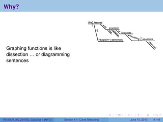
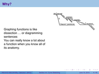
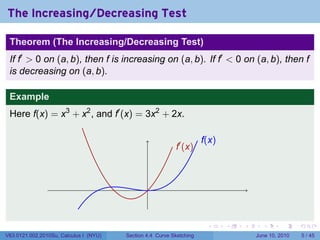
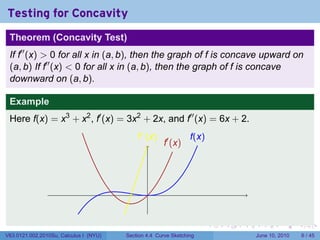
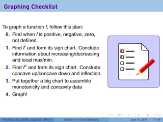
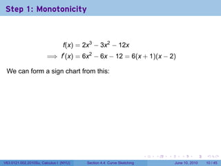
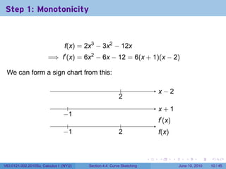
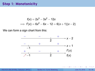
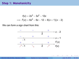
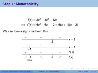
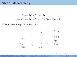
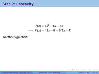
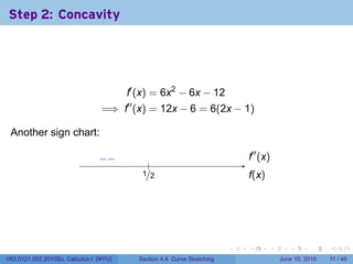
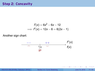
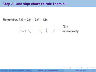
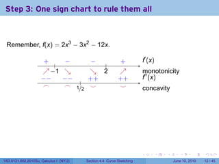
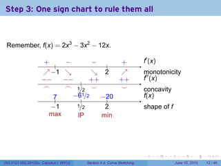
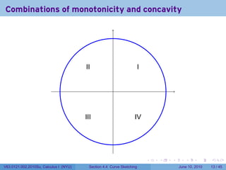
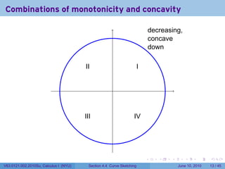
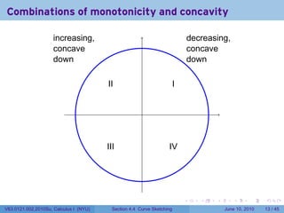
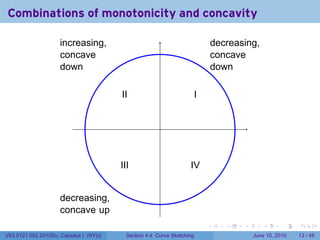
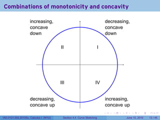
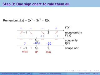
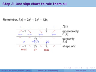
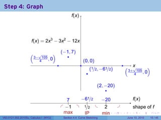
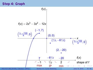
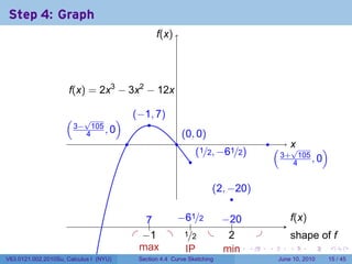
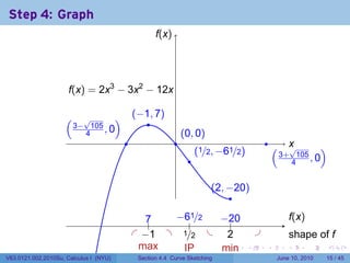
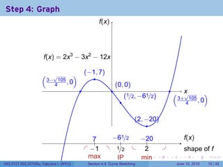
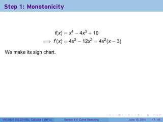
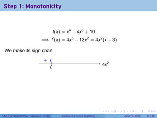
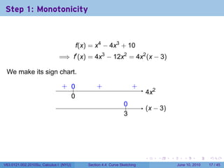
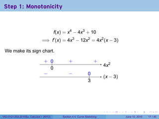
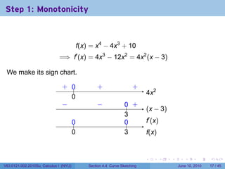
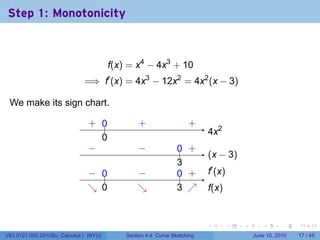
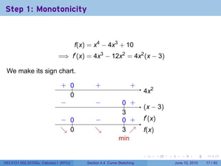
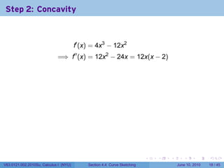
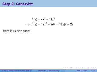
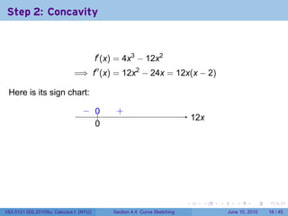
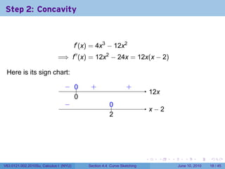
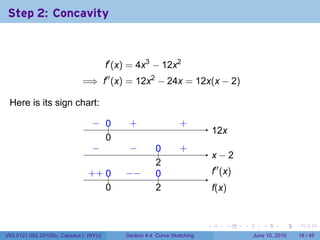
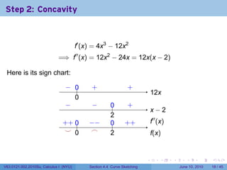
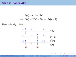
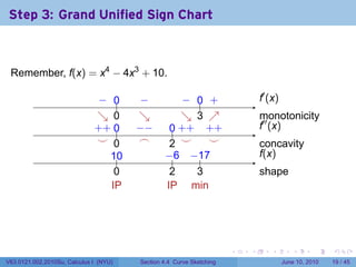
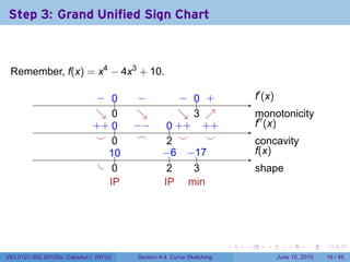
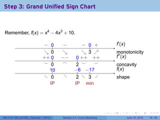
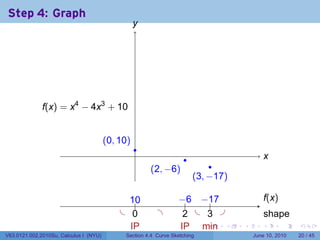
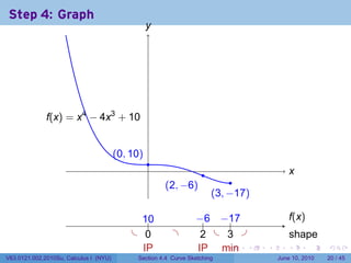
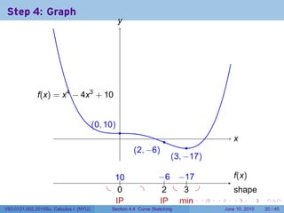
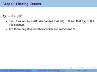
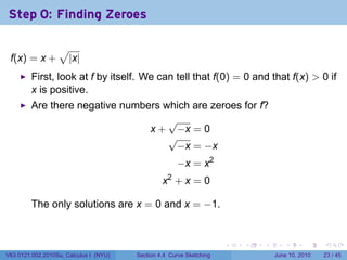
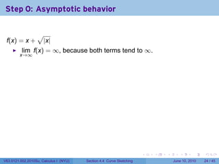
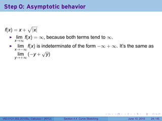
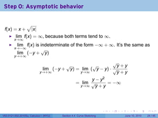
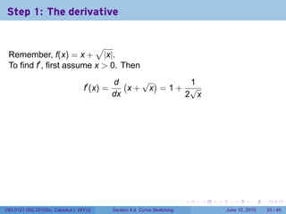
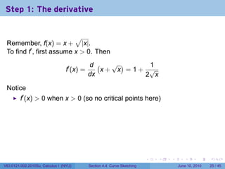
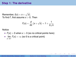
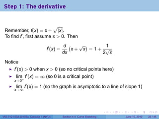
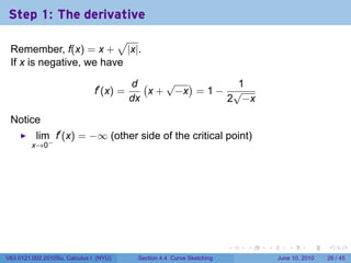
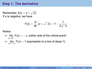
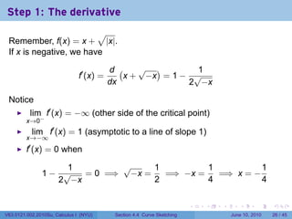
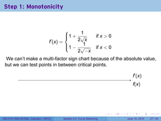
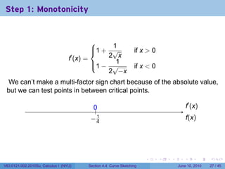
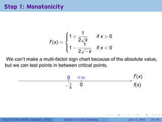
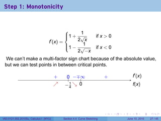
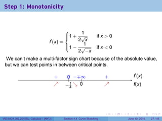
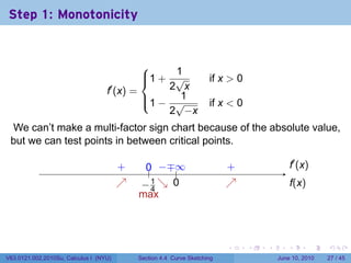
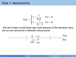
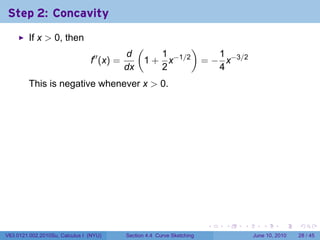
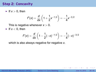
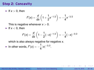
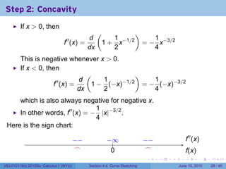
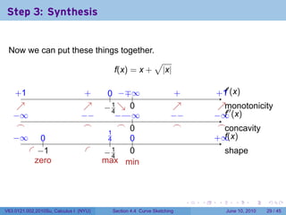
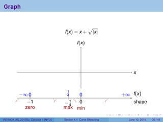
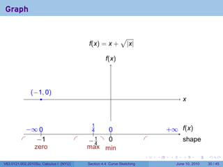
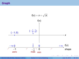
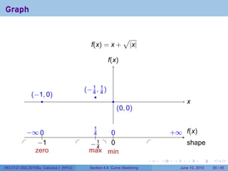
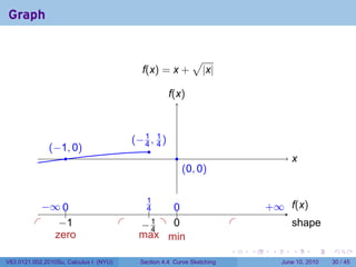
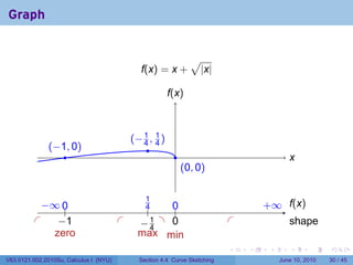
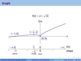
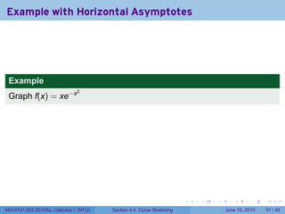
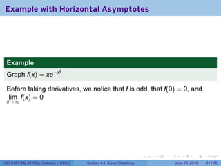
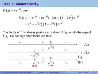
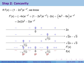
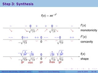
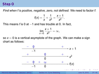
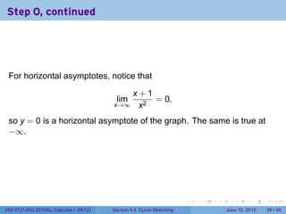
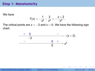
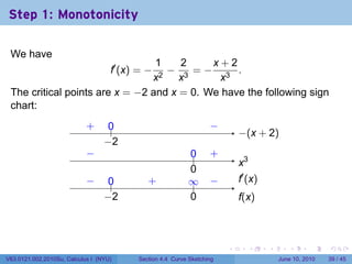
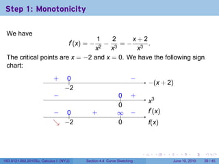
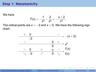
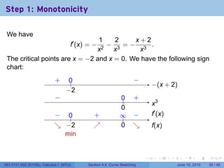
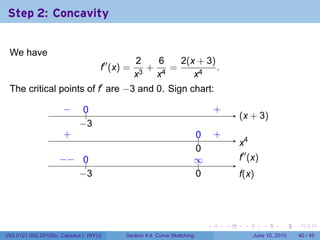
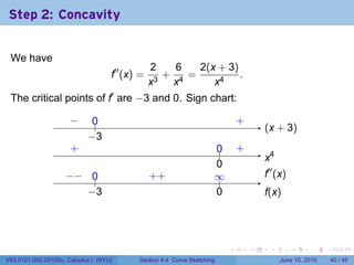
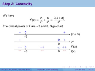
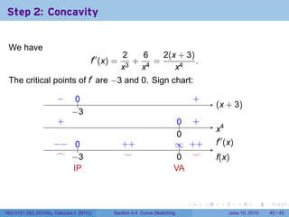
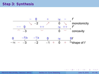
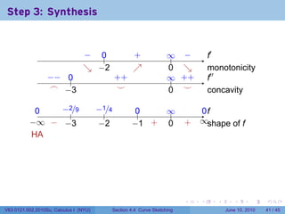
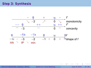
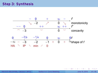
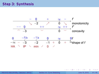
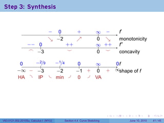
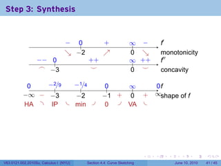
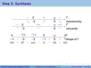
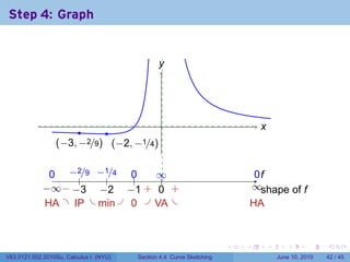
The document provides an overview of curve sketching in calculus. It discusses objectives like sketching a function graph completely by identifying zeros, asymptotes, critical points, maxima/minima and inflection points. Examples are provided to demonstrate the increasing/decreasing test using derivatives and the concavity test to determine concave up/down regions. A step-by-step process is outlined to graph functions which involves analyzing monotonicity using the sign chart of the derivative and concavity using the second derivative sign chart. This is demonstrated on sketching the graph of a cubic function f(x)=2x^3-3x^2-12x.

1. Section 4.4
Curve Sketching
V63.0121.002.2010Su, Calculus I
New York University
June 10, 2010
Announcements
Homework 4 due Tuesday
. . . . . .

2. Announcements
Homework 4 due Tuesday
. . . . . .
V63.0121.002.2010Su, Calculus I (NYU) Section 4.4 Curve Sketching June 10, 2010 2 / 45

3. Objectives
given a function, graph it
completely, indicating
zeroes (if easy)
asymptotes if applicable
critical points
local/global max/min
inflection points
. . . . . .
V63.0121.002.2010Su, Calculus I (NYU) Section 4.4 Curve Sketching June 10, 2010 3 / 45

4. Why?
Graphing functions is like
dissection
. . . . . .
V63.0121.002.2010Su, Calculus I (NYU) Section 4.4 Curve Sketching June 10, 2010 4 / 45

5. Why?
Graphing functions is like
dissection … or diagramming
sentences
. . . . . .
V63.0121.002.2010Su, Calculus I (NYU) Section 4.4 Curve Sketching June 10, 2010 4 / 45

6. Why?
Graphing functions is like
dissection … or diagramming
sentences
You can really know a lot about
a function when you know all of
its anatomy.
. . . . . .
V63.0121.002.2010Su, Calculus I (NYU) Section 4.4 Curve Sketching June 10, 2010 4 / 45

7. The Increasing/Decreasing Test
Theorem (The Increasing/Decreasing Test)
If f′ > 0 on (a, b), then f is increasing on (a, b). If f′ < 0 on (a, b), then f
is decreasing on (a, b).
Example
Here f(x) = x3 + x2 , and f′ (x) = 3x2 + 2x.
f
.(x)
.′ (x)
f
.
. . . . . .
V63.0121.002.2010Su, Calculus I (NYU) Section 4.4 Curve Sketching June 10, 2010 5 / 45

8. Testing for Concavity
Theorem (Concavity Test)
If f′′ (x) > 0 for all x in (a, b), then the graph of f is concave upward on
(a, b) If f′′ (x) < 0 for all x in (a, b), then the graph of f is concave
downward on (a, b).
Example
Here f(x) = x3 + x2 , f′ (x) = 3x2 + 2x, and f′′ (x) = 6x + 2.
.′′ (x)
f f
.(x)
.′ (x)
f
.
. . . . . .
V63.0121.002.2010Su, Calculus I (NYU) Section 4.4 Curve Sketching June 10, 2010 6 / 45

9. Graphing Checklist
To graph a function f, follow this plan:
0. Find when f is positive, negative, zero,
not defined.
1. Find f′ and form its sign chart. Conclude
information about increasing/decreasing
and local max/min.
2. Find f′′ and form its sign chart. Conclude
concave up/concave down and inflection.
3. Put together a big chart to assemble
monotonicity and concavity data
4. Graph!
. . . . . .
V63.0121.002.2010Su, Calculus I (NYU) Section 4.4 Curve Sketching June 10, 2010 7 / 45

10. Outline
Simple examples
A cubic function
A quartic function
More Examples
Points of nondifferentiability
Horizontal asymptotes
Vertical asymptotes
Trigonometric and polynomial together
Logarithmic
. . . . . .
V63.0121.002.2010Su, Calculus I (NYU) Section 4.4 Curve Sketching June 10, 2010 8 / 45

11. Graphing a cubic
Example
Graph f(x) = 2x3 − 3x2 − 12x.
. . . . . .
V63.0121.002.2010Su, Calculus I (NYU) Section 4.4 Curve Sketching June 10, 2010 9 / 45

12. Graphing a cubic
Example
Graph f(x) = 2x3 − 3x2 − 12x.
(Step 0) First, let’s find the zeros. We can at least factor out one power
of x:
f(x) = x(2x2 − 3x − 12)
so f(0) = 0. The other factor is a quadratic, so we the other two roots
are √
√
3 ± 32 − 4(2)(−12) 3 ± 105
x= =
4 4
It’s OK to skip this step for now since the roots are so complicated.
. . . . . .
V63.0121.002.2010Su, Calculus I (NYU) Section 4.4 Curve Sketching June 10, 2010 9 / 45

13. Step 1: Monotonicity
f(x) = 2x3 − 3x2 − 12x
=⇒ f′ (x) = 6x2 − 6x − 12 = 6(x + 1)(x − 2)
We can form a sign chart from this:
.
. . . . . .
V63.0121.002.2010Su, Calculus I (NYU) Section 4.4 Curve Sketching June 10, 2010 10 / 45

14. Step 1: Monotonicity
f(x) = 2x3 − 3x2 − 12x
=⇒ f′ (x) = 6x2 − 6x − 12 = 6(x + 1)(x − 2)
We can form a sign chart from this:
. . . −2
x
2
.
. x
. +1
−
. 1
.′ (x)
f
. .
−
. 1 2
. f
.(x)
. . . . . .
V63.0121.002.2010Su, Calculus I (NYU) Section 4.4 Curve Sketching June 10, 2010 10 / 45

15. Step 1: Monotonicity
f(x) = 2x3 − 3x2 − 12x
=⇒ f′ (x) = 6x2 − 6x − 12 = 6(x + 1)(x − 2)
We can form a sign chart from this:
−
. −
. . . .
+
. −2
x
2
.
. x
. +1
−
. 1
.′ (x)
f
. .
−
. 1 2
. f
.(x)
. . . . . .
V63.0121.002.2010Su, Calculus I (NYU) Section 4.4 Curve Sketching June 10, 2010 10 / 45

16. Step 1: Monotonicity
f(x) = 2x3 − 3x2 − 12x
=⇒ f′ (x) = 6x2 − 6x − 12 = 6(x + 1)(x − 2)
We can form a sign chart from this:
−
. −
. . . .
+
. −2
x
2
.
−
. . .
+ .
+
x
. +1
−
. 1
.′ (x)
f
. .
−
. 1 2
. f
.(x)
. . . . . .
V63.0121.002.2010Su, Calculus I (NYU) Section 4.4 Curve Sketching June 10, 2010 10 / 45

17. Step 1: Monotonicity
f(x) = 2x3 − 3x2 − 12x
=⇒ f′ (x) = 6x2 − 6x − 12 = 6(x + 1)(x − 2)
We can form a sign chart from this:
−
. −
. . . .
+
. −2
x
2
.
−
. . .
+ .
+
x
. +1
−
. 1
. .
+ .′ (x)
f
.
−
. 1 2
. f
.(x)
. . . . . .
V63.0121.002.2010Su, Calculus I (NYU) Section 4.4 Curve Sketching June 10, 2010 10 / 45

18. Step 1: Monotonicity
f(x) = 2x3 − 3x2 − 12x
=⇒ f′ (x) = 6x2 − 6x − 12 = 6(x + 1)(x − 2)
We can form a sign chart from this:
−
. −
. . . .
+
. −2
x
2
.
−
. . .
+ .
+
x
. +1
−
. 1
. .
+ −
. .′ (x)
f
.
−
. 1 2
. f
.(x)
. . . . . .
V63.0121.002.2010Su, Calculus I (NYU) Section 4.4 Curve Sketching June 10, 2010 10 / 45

19. Step 1: Monotonicity
f(x) = 2x3 − 3x2 − 12x
=⇒ f′ (x) = 6x2 − 6x − 12 = 6(x + 1)(x − 2)
We can form a sign chart from this:
−
. −
. . . .
+
. −2
x
2
.
−
. . .
+ .
+
x
. +1
−
. 1
. .
+ −
. .
+ .′ (x)
f
.
−
. 1 2
. f
.(x)
. . . . . .
V63.0121.002.2010Su, Calculus I (NYU) Section 4.4 Curve Sketching June 10, 2010 10 / 45

20. Step 1: Monotonicity
f(x) = 2x3 − 3x2 − 12x
=⇒ f′ (x) = 6x2 − 6x − 12 = 6(x + 1)(x − 2)
We can form a sign chart from this:
−
. −
. . . .
+
. −2
x
2
.
−
. . .
+ .
+
x
. +1
−
. 1
. .
+ −
. .
+ .′ (x)
f
.
↗−
. . 1 2
. f
.(x)
. . . . . .
V63.0121.002.2010Su, Calculus I (NYU) Section 4.4 Curve Sketching June 10, 2010 10 / 45

21. Step 1: Monotonicity
f(x) = 2x3 − 3x2 − 12x
=⇒ f′ (x) = 6x2 − 6x − 12 = 6(x + 1)(x − 2)
We can form a sign chart from this:
−
. −
. . . .
+
. −2
x
2
.
−
. . .
+ .
+
x
. +1
−
. 1
. .
+ −
. .
+ .′ (x)
f
.
↗−
. . 1 ↘
. 2
. f
.(x)
. . . . . .
V63.0121.002.2010Su, Calculus I (NYU) Section 4.4 Curve Sketching June 10, 2010 10 / 45

22. Step 1: Monotonicity
f(x) = 2x3 − 3x2 − 12x
=⇒ f′ (x) = 6x2 − 6x − 12 = 6(x + 1)(x − 2)
We can form a sign chart from this:
−
. −
. . . .
+
. −2
x
2
.
−
. . .
+ .
+
x
. +1
−
. 1
. .
+ −
. .
+ .′ (x)
f
.
↗−
. . 1 ↘
. 2
. ↗
. f
.(x)
. . . . . .
V63.0121.002.2010Su, Calculus I (NYU) Section 4.4 Curve Sketching June 10, 2010 10 / 45

23. Step 1: Monotonicity
f(x) = 2x3 − 3x2 − 12x
=⇒ f′ (x) = 6x2 − 6x − 12 = 6(x + 1)(x − 2)
We can form a sign chart from this:
−
. −
. . . .
+
. −2
x
2
.
−
. . .
+ .
+
x
. +1
−
. 1
. .
+ −
. .
+ .′ (x)
f
.
↗−
. . 1 ↘
. 2
. ↗
. f
.(x)
m
. ax
. . . . . .
V63.0121.002.2010Su, Calculus I (NYU) Section 4.4 Curve Sketching June 10, 2010 10 / 45

24. Step 1: Monotonicity
f(x) = 2x3 − 3x2 − 12x
=⇒ f′ (x) = 6x2 − 6x − 12 = 6(x + 1)(x − 2)
We can form a sign chart from this:
−
. −
. . . .
+
. −2
x
2
.
−
. . .
+ .
+
x
. +1
−
. 1
. .
+ −
. .
+ .′ (x)
f
.
↗−
. . 1 ↘
. 2
. ↗
. f
.(x)
m
. ax m
. in
. . . . . .
V63.0121.002.2010Su, Calculus I (NYU) Section 4.4 Curve Sketching June 10, 2010 10 / 45

25. Step 2: Concavity
f′ (x) = 6x2 − 6x − 12
=⇒ f′′ (x) = 12x − 6 = 6(2x − 1)
Another sign chart: .
. . . . . .
V63.0121.002.2010Su, Calculus I (NYU) Section 4.4 Curve Sketching June 10, 2010 11 / 45

26. Step 2: Concavity
f′ (x) = 6x2 − 6x − 12
=⇒ f′′ (x) = 12x − 6 = 6(2x − 1)
Another sign chart: .
.′′ (x)
f
.
./2
1 f
.(x)
. . . . . .
V63.0121.002.2010Su, Calculus I (NYU) Section 4.4 Curve Sketching June 10, 2010 11 / 45

27. Step 2: Concavity
f′ (x) = 6x2 − 6x − 12
=⇒ f′′ (x) = 12x − 6 = 6(2x − 1)
Another sign chart: .
−
. − .′′ (x)
f
.
./2
1 f
.(x)
. . . . . .
V63.0121.002.2010Su, Calculus I (NYU) Section 4.4 Curve Sketching June 10, 2010 11 / 45

28. Step 2: Concavity
f′ (x) = 6x2 − 6x − 12
=⇒ f′′ (x) = 12x − 6 = 6(2x − 1)
Another sign chart: .
−
. − . +
+ .′′ (x)
f
.
./2
1 f
.(x)
. . . . . .
V63.0121.002.2010Su, Calculus I (NYU) Section 4.4 Curve Sketching June 10, 2010 11 / 45

29. Step 2: Concavity
f′ (x) = 6x2 − 6x − 12
=⇒ f′′ (x) = 12x − 6 = 6(2x − 1)
Another sign chart: .
−
. − . +
+ .′′ (x)
f
.
.
⌢ ./2
1 f
.(x)
. . . . . .
V63.0121.002.2010Su, Calculus I (NYU) Section 4.4 Curve Sketching June 10, 2010 11 / 45

30. Step 2: Concavity
f′ (x) = 6x2 − 6x − 12
=⇒ f′′ (x) = 12x − 6 = 6(2x − 1)
Another sign chart: .
−
. − . +
+ .′′ (x)
f
.
.
⌢ ./2
1 .
⌣ f
.(x)
. . . . . .
V63.0121.002.2010Su, Calculus I (NYU) Section 4.4 Curve Sketching June 10, 2010 11 / 45

31. Step 2: Concavity
f′ (x) = 6x2 − 6x − 12
=⇒ f′′ (x) = 12x − 6 = 6(2x − 1)
Another sign chart: .
−
. − . +
+ .′′ (x)
f
.
.
⌢ ./2
1 .
⌣ f
.(x)
I
.P
. . . . . .
V63.0121.002.2010Su, Calculus I (NYU) Section 4.4 Curve Sketching June 10, 2010 11 / 45

32. Step 3: One sign chart to rule them all
Remember, f(x) = 2x3 − 3x2 − 12x.
.
. . . . . .
V63.0121.002.2010Su, Calculus I (NYU) Section 4.4 Curve Sketching June 10, 2010 12 / 45

33. Step 3: One sign chart to rule them all
Remember, f(x) = 2x3 − 3x2 − 12x.
−
. . . .
+ −
. .
+ .′ (x)
f
.
↗− ↘
. . 1 . ↘
. 2
. ↗
. m
. onotonicity
. . . . . .
V63.0121.002.2010Su, Calculus I (NYU) Section 4.4 Curve Sketching June 10, 2010 12 / 45

34. Step 3: One sign chart to rule them all
Remember, f(x) = 2x3 − 3x2 − 12x.
. .
+ −
. . −
. .
+ .′ (x)
f
.
↗−
. . 1 ↘
. ↘ .
. 2 ↗
. m
.′′ onotonicity
−
. − −
. − . . +
+ . +
+ f
. (x)
.
⌢ .
⌢ 1/2
. .
⌣ .
⌣ c
. oncavity
. . . . . .
V63.0121.002.2010Su, Calculus I (NYU) Section 4.4 Curve Sketching June 10, 2010 12 / 45

35. Step 3: One sign chart to rule them all
Remember, f(x) = 2x3 − 3x2 − 12x.
. .
+ −
. . −
. .
+ .′ (x)
f
.
↗−
. . 1 ↘
. ↘ .
. 2 ↗
. m
.′′ onotonicity
−
. − −
. − . . + + . +
+ f
. (x)
.
⌢ ⌢ ./2 .
. 1 ⌣ .
⌣ c
. oncavity
7
.. −
. 6 1/2 −.
. 20 f
.(x)
.
−
. 1 .
1/2 2
. s
. hape of f
m
. ax I
.P m
. in
. . . . . .
V63.0121.002.2010Su, Calculus I (NYU) Section 4.4 Curve Sketching June 10, 2010 12 / 45

36. Combinations of monotonicity and concavity
I
.I I
.
.
I
.II I
.V
. . . . . .
V63.0121.002.2010Su, Calculus I (NYU) Section 4.4 Curve Sketching June 10, 2010 13 / 45

37. Combinations of monotonicity and concavity
.
decreasing,
concave
down
I
.I I
.
.
I
.II I
.V
. . . . . .
V63.0121.002.2010Su, Calculus I (NYU) Section 4.4 Curve Sketching June 10, 2010 13 / 45

38. Combinations of monotonicity and concavity
. .
increasing, decreasing,
concave concave
down down
I
.I I
.
.
I
.II I
.V
. . . . . .
V63.0121.002.2010Su, Calculus I (NYU) Section 4.4 Curve Sketching June 10, 2010 13 / 45

39. Combinations of monotonicity and concavity
. .
increasing, decreasing,
concave concave
down down
I
.I I
.
.
I
.II I
.V
.
decreasing,
concave up
. . . . . .
V63.0121.002.2010Su, Calculus I (NYU) Section 4.4 Curve Sketching June 10, 2010 13 / 45

40. Combinations of monotonicity and concavity
. .
increasing, decreasing,
concave concave
down down
I
.I I
.
.
I
.II I
.V
. .
decreasing, increasing,
concave up concave up
. . . . . .
V63.0121.002.2010Su, Calculus I (NYU) Section 4.4 Curve Sketching June 10, 2010 13 / 45

41. Step 3: One sign chart to rule them all
Remember, f(x) = 2x3 − 3x2 − 12x.
. .
+ −
. . −
. .
+ .′ (x)
f
.
↗−
. . 1 ↘
. ↘ .
. 2 ↗
. m
.′′ onotonicity
−
. − −
. − . . + + . +
+ f
. (x)
.
⌢ ⌢ ./2 .
. 1 ⌣ .
⌣ c
. oncavity
7
.. −
. 6 1/2 −.
. 20 f
.(x)
.
. . 1
− .
1/2 2
. s
. hape of f
m
. ax I
.P m
. in
. . . . . .
V63.0121.002.2010Su, Calculus I (NYU) Section 4.4 Curve Sketching June 10, 2010 14 / 45

42. Step 3: One sign chart to rule them all
Remember, f(x) = 2x3 − 3x2 − 12x.
. .
+ −
. . −
. .
+ .′ (x)
f
.
↗−
. . 1 ↘
. ↘ .
. 2 ↗
. m
.′′ onotonicity
−
. − −
. − . . + + . +
+ f
. (x)
.
⌢ ⌢ ./2 .
. 1 ⌣ .
⌣ c
. oncavity
7
.. −
. 6 1/2 −.
. 20 f
.(x)
.
. . 1 . ./2
− 1 2
. s
. hape of f
m
. ax I
.P m
. in
. . . . . .
V63.0121.002.2010Su, Calculus I (NYU) Section 4.4 Curve Sketching June 10, 2010 14 / 45

43. Step 3: One sign chart to rule them all
Remember, f(x) = 2x3 − 3x2 − 12x.
. .
+ −
. . −
. .
+ .′ (x)
f
.
↗−
. . 1 ↘
. ↘ .
. 2 ↗
. m
.′′ onotonicity
−
. − −
. − . . + + . +
+ f
. (x)
.
⌢ ⌢ ./2 .
. 1 ⌣ .
⌣ c
. oncavity
7
.. −
. 6 1/2 −.
. 20 f
.(x)
.
. . 1 . ./2 .
− 1 2
. s
. hape of f
m
. ax I
.P m
. in
. . . . . .
V63.0121.002.2010Su, Calculus I (NYU) Section 4.4 Curve Sketching June 10, 2010 14 / 45

44. Step 3: One sign chart to rule them all
Remember, f(x) = 2x3 − 3x2 − 12x.
. .
+ −
. . −
. .
+ .′ (x)
f
.
↗−
. . 1 ↘
. ↘ .
. 2 ↗
. m
.′′ onotonicity
−
. − −
. − . . + + . +
+ f
. (x)
.
⌢ ⌢ ./2 .
. 1 ⌣ .
⌣ c
. oncavity
7
.. −
. 6 1/2 −.
. 20 f
.(x)
.
. . 1 . ./2 .
− 1 2
. . s
. hape of f
m
. ax I
.P m
. in
. . . . . .
V63.0121.002.2010Su, Calculus I (NYU) Section 4.4 Curve Sketching June 10, 2010 14 / 45

45. Step 4: Graph
f
.(x)
.(x) = 2x3 − 3x2 − 12x
f
( √ ) . −1, 7)
(
.
. 3− 4105 , 0 . 0, 0)
(
. . .
. 1/2, −61/2)
( ( . x
√ )
. . 3+ 4105 , 0
. 2, −20)
(
.
7
.. −
. 61/2 −.
. 20 f
.(x)
.
. . 1 . ./2 .
− 1 2
. . s
. hape of f
m
. ax I
.P m
. in . . . . . .
V63.0121.002.2010Su, Calculus I (NYU) Section 4.4 Curve Sketching June 10, 2010 15 / 45

46. Step 4: Graph
f
.(x)
.(x) = 2x3 − 3x2 − 12x
f
( √ ) . −1, 7)
(
.
. 3− 4105 , 0 . 0, 0)
(
. . .
. 1/2, −61/2)
( ( . x
√ )
. . 3+ 4105 , 0
. 2, −20)
(
.
7
.. −
. 61/2 −.
. 20 f
.(x)
.
. . 1 . ./2 .
− 1 2
. . s
. hape of f
m
. ax I
.P m
. in . . . . . .
V63.0121.002.2010Su, Calculus I (NYU) Section 4.4 Curve Sketching June 10, 2010 15 / 45

47. Step 4: Graph
f
.(x)
.(x) = 2x3 − 3x2 − 12x
f
( √ ) . −1, 7)
(
.
. 3− 4105 , 0 . 0, 0)
(
. . .
. 1/2, −61/2)
( ( . x
√ )
. . 3+ 4105 , 0
. 2, −20)
(
.
7
.. −
. 61/2 −.
. 20 f
.(x)
.
. . 1 . ./2 .
− 1 2
. . s
. hape of f
m
. ax I
.P m
. in . . . . . .
V63.0121.002.2010Su, Calculus I (NYU) Section 4.4 Curve Sketching June 10, 2010 15 / 45

48. Step 4: Graph
f
.(x)
.(x) = 2x3 − 3x2 − 12x
f
( √ ) . −1, 7)
(
.
. 3− 4105 , 0 . 0, 0)
(
. . .
. 1/2, −61/2)
( ( . x
√ )
. . 3+ 4105 , 0
. 2, −20)
(
.
7
.. −
. 61/2 −.
. 20 f
.(x)
.
. . 1 . ./2 .
− 1 2
. . s
. hape of f
m
. ax I
.P m
. in . . . . . .
V63.0121.002.2010Su, Calculus I (NYU) Section 4.4 Curve Sketching June 10, 2010 15 / 45

49. Step 4: Graph
f
.(x)
.(x) = 2x3 − 3x2 − 12x
f
( √ ) . −1, 7)
(
.
. 3− 4105 , 0 . 0, 0)
(
. . .
. 1/2, −61/2)
( ( . x
√ )
. . 3+ 4105 , 0
. 2, −20)
(
.
7
.. −
. 61/2 −.
. 20 f
.(x)
.
. . 1 . ./2 .
− 1 2
. . s
. hape of f
m
. ax I
.P m
. in . . . . . .
V63.0121.002.2010Su, Calculus I (NYU) Section 4.4 Curve Sketching June 10, 2010 15 / 45

50. Graphing a quartic
Example
Graph f(x) = x4 − 4x3 + 10
. . . . . .
V63.0121.002.2010Su, Calculus I (NYU) Section 4.4 Curve Sketching June 10, 2010 16 / 45

51. Graphing a quartic
Example
Graph f(x) = x4 − 4x3 + 10
(Step 0) We know f(0) = 10 and lim f(x) = +∞. Not too many other
x→±∞
points on the graph are evident.
. . . . . .
V63.0121.002.2010Su, Calculus I (NYU) Section 4.4 Curve Sketching June 10, 2010 16 / 45

52. Step 1: Monotonicity
f(x) = x4 − 4x3 + 10
=⇒ f′ (x) = 4x3 − 12x2 = 4x2 (x − 3)
. . . . . .
V63.0121.002.2010Su, Calculus I (NYU) Section 4.4 Curve Sketching June 10, 2010 17 / 45

53. Step 1: Monotonicity
f(x) = x4 − 4x3 + 10
=⇒ f′ (x) = 4x3 − 12x2 = 4x2 (x − 3)
We make its sign chart.
.
. . . . . .
V63.0121.002.2010Su, Calculus I (NYU) Section 4.4 Curve Sketching June 10, 2010 17 / 45

54. Step 1: Monotonicity
f(x) = x4 − 4x3 + 10
=⇒ f′ (x) = 4x3 − 12x2 = 4x2 (x − 3)
We make its sign chart.
0
..
. x2
4
0
.
. . . . . .
V63.0121.002.2010Su, Calculus I (NYU) Section 4.4 Curve Sketching June 10, 2010 17 / 45

55. Step 1: Monotonicity
f(x) = x4 − 4x3 + 10
=⇒ f′ (x) = 4x3 − 12x2 = 4x2 (x − 3)
We make its sign chart.
. ..
+ 0
. x2
4
0
.
. . . . . .
V63.0121.002.2010Su, Calculus I (NYU) Section 4.4 Curve Sketching June 10, 2010 17 / 45

56. Step 1: Monotonicity
f(x) = x4 − 4x3 + 10
=⇒ f′ (x) = 4x3 − 12x2 = 4x2 (x − 3)
We make its sign chart.
. ..
+ 0 .
+
. x2
4
0
.
. . . . . .
V63.0121.002.2010Su, Calculus I (NYU) Section 4.4 Curve Sketching June 10, 2010 17 / 45

57. Step 1: Monotonicity
f(x) = x4 − 4x3 + 10
=⇒ f′ (x) = 4x3 − 12x2 = 4x2 (x − 3)
We make its sign chart.
. ..
+ 0 .
+ .
+
. x2
4
0
.
. . . . . .
V63.0121.002.2010Su, Calculus I (NYU) Section 4.4 Curve Sketching June 10, 2010 17 / 45

58. Step 1: Monotonicity
f(x) = x4 − 4x3 + 10
=⇒ f′ (x) = 4x3 − 12x2 = 4x2 (x − 3)
We make its sign chart.
. ..
+ 0 .
+ .
+
. x2
4
0
.
0
..
. x − 3)
(
3
.
. . . . . .
V63.0121.002.2010Su, Calculus I (NYU) Section 4.4 Curve Sketching June 10, 2010 17 / 45

59. Step 1: Monotonicity
f(x) = x4 − 4x3 + 10
=⇒ f′ (x) = 4x3 − 12x2 = 4x2 (x − 3)
We make its sign chart.
. ..
+ 0 .
+ .
+
. x2
4
0
.
−
. 0
..
. x − 3)
(
3
.
. . . . . .
V63.0121.002.2010Su, Calculus I (NYU) Section 4.4 Curve Sketching June 10, 2010 17 / 45

60. Step 1: Monotonicity
f(x) = x4 − 4x3 + 10
=⇒ f′ (x) = 4x3 − 12x2 = 4x2 (x − 3)
We make its sign chart.
. ..
+ 0 .
+ .
+
. x2
4
0
.
−
. −
. 0
..
. x − 3)
(
3
.
. . . . . .
V63.0121.002.2010Su, Calculus I (NYU) Section 4.4 Curve Sketching June 10, 2010 17 / 45

61. Step 1: Monotonicity
f(x) = x4 − 4x3 + 10
=⇒ f′ (x) = 4x3 − 12x2 = 4x2 (x − 3)
We make its sign chart.
. ..
+ 0 .
+ .
+
. x2
4
0
.
−
. −
. .. .
0 +
. x − 3)
(
3
.
. . . . . .
V63.0121.002.2010Su, Calculus I (NYU) Section 4.4 Curve Sketching June 10, 2010 17 / 45

62. Step 1: Monotonicity
f(x) = x4 − 4x3 + 10
=⇒ f′ (x) = 4x3 − 12x2 = 4x2 (x − 3)
We make its sign chart.
. ..
+ 0 .
+ .
+
. x2
4
0
.
−
. −
. .. .
0 +
. x − 3)
(
3
.
0
.. 0
.. .′ (x)
f
0
. 3
. f
.(x)
. . . . . .
V63.0121.002.2010Su, Calculus I (NYU) Section 4.4 Curve Sketching June 10, 2010 17 / 45

63. Step 1: Monotonicity
f(x) = x4 − 4x3 + 10
=⇒ f′ (x) = 4x3 − 12x2 = 4x2 (x − 3)
We make its sign chart.
. ..
+ 0 .
+ .
+
. x2
4
0
.
−
. −
. .. .
0 +
. x − 3)
(
3
.
− 0
. .. 0
.. .′ (x)
f
0
. 3
. f
.(x)
. . . . . .
V63.0121.002.2010Su, Calculus I (NYU) Section 4.4 Curve Sketching June 10, 2010 17 / 45

64. Step 1: Monotonicity
f(x) = x4 − 4x3 + 10
=⇒ f′ (x) = 4x3 − 12x2 = 4x2 (x − 3)
We make its sign chart.
. ..
+ 0 .
+ .
+
. x2
4
0
.
−
. −
. .. .
0 +
. x − 3)
(
3
.
− 0
. .. −
. 0
.. .′ (x)
f
0
. 3
. f
.(x)
. . . . . .
V63.0121.002.2010Su, Calculus I (NYU) Section 4.4 Curve Sketching June 10, 2010 17 / 45

65. Step 1: Monotonicity
f(x) = x4 − 4x3 + 10
=⇒ f′ (x) = 4x3 − 12x2 = 4x2 (x − 3)
We make its sign chart.
. ..
+ 0 .
+ .
+
. x2
4
0
.
−
. −
. .. .
0 +
. x − 3)
(
3
.
− 0
. .. −
. .. .
0 + .′ (x)
f
0
. 3
. f
.(x)
. . . . . .
V63.0121.002.2010Su, Calculus I (NYU) Section 4.4 Curve Sketching June 10, 2010 17 / 45

66. Step 1: Monotonicity
f(x) = x4 − 4x3 + 10
=⇒ f′ (x) = 4x3 − 12x2 = 4x2 (x − 3)
We make its sign chart.
. ..
+ 0 .
+ .
+
. x2
4
0
.
−
. −
. .. .
0 +
. x − 3)
(
3
.
− 0
. .. −
. .. .
0 + .′ (x)
f
↘ 0
. . 3
. f
.(x)
. . . . . .
V63.0121.002.2010Su, Calculus I (NYU) Section 4.4 Curve Sketching June 10, 2010 17 / 45

67. Step 1: Monotonicity
f(x) = x4 − 4x3 + 10
=⇒ f′ (x) = 4x3 − 12x2 = 4x2 (x − 3)
We make its sign chart.
. ..
+ 0 .
+ .
+
. x2
4
0
.
−
. −
. .. .
0 +
. x − 3)
(
3
.
− 0
. .. −
. .. .
0 + .′ (x)
f
↘ 0
. . ↘
. 3
. f
.(x)
. . . . . .
V63.0121.002.2010Su, Calculus I (NYU) Section 4.4 Curve Sketching June 10, 2010 17 / 45

68. Step 1: Monotonicity
f(x) = x4 − 4x3 + 10
=⇒ f′ (x) = 4x3 − 12x2 = 4x2 (x − 3)
We make its sign chart.
. ..
+ 0 .
+ .
+
. x2
4
0
.
−
. −
. .. .
0 +
. x − 3)
(
3
.
− 0
. .. −
. .. .
0 + .′ (x)
f
↘ 0
. . ↘
. 3 ↗
. . f
.(x)
. . . . . .
V63.0121.002.2010Su, Calculus I (NYU) Section 4.4 Curve Sketching June 10, 2010 17 / 45

69. Step 1: Monotonicity
f(x) = x4 − 4x3 + 10
=⇒ f′ (x) = 4x3 − 12x2 = 4x2 (x − 3)
We make its sign chart.
. ..
+ 0 .
+ .
+
. x2
4
0
.
−
. −
. .. .
0 +
. x − 3)
(
3
.
− 0
. .. −
. .. .
0 + .′ (x)
f
↘ 0
. . ↘
. 3 ↗
. . f
.(x)
m
. in
. . . . . .
V63.0121.002.2010Su, Calculus I (NYU) Section 4.4 Curve Sketching June 10, 2010 17 / 45

70. Step 2: Concavity
f′ (x) = 4x3 − 12x2
=⇒ f′′ (x) = 12x2 − 24x = 12x(x − 2)
.
. . . . . .
V63.0121.002.2010Su, Calculus I (NYU) Section 4.4 Curve Sketching June 10, 2010 18 / 45

71. Step 2: Concavity
f′ (x) = 4x3 − 12x2
=⇒ f′′ (x) = 12x2 − 24x = 12x(x − 2)
Here is its sign chart:
.
. . . . . .
V63.0121.002.2010Su, Calculus I (NYU) Section 4.4 Curve Sketching June 10, 2010 18 / 45

72. Step 2: Concavity
f′ (x) = 4x3 − 12x2
=⇒ f′′ (x) = 12x2 − 24x = 12x(x − 2)
Here is its sign chart:
0
..
1
. 2x
0
.
. . . . . .
V63.0121.002.2010Su, Calculus I (NYU) Section 4.4 Curve Sketching June 10, 2010 18 / 45

73. Step 2: Concavity
f′ (x) = 4x3 − 12x2
=⇒ f′′ (x) = 12x2 − 24x = 12x(x − 2)
Here is its sign chart:
− 0
. ..
1
. 2x
0
.
. . . . . .
V63.0121.002.2010Su, Calculus I (NYU) Section 4.4 Curve Sketching June 10, 2010 18 / 45

74. Step 2: Concavity
f′ (x) = 4x3 − 12x2
=⇒ f′′ (x) = 12x2 − 24x = 12x(x − 2)
Here is its sign chart:
− 0
. .. .
+
1
. 2x
0
.
. . . . . .
V63.0121.002.2010Su, Calculus I (NYU) Section 4.4 Curve Sketching June 10, 2010 18 / 45

75. Step 2: Concavity
f′ (x) = 4x3 − 12x2
=⇒ f′′ (x) = 12x2 − 24x = 12x(x − 2)
Here is its sign chart:
− 0
. .. .
+ .
+
1
. 2x
0
.
. . . . . .
V63.0121.002.2010Su, Calculus I (NYU) Section 4.4 Curve Sketching June 10, 2010 18 / 45

76. Step 2: Concavity
f′ (x) = 4x3 − 12x2
=⇒ f′′ (x) = 12x2 − 24x = 12x(x − 2)
Here is its sign chart:
− 0
. .. .
+ .
+
1
. 2x
0
.
0
..
. −2
x
2
.
. . . . . .
V63.0121.002.2010Su, Calculus I (NYU) Section 4.4 Curve Sketching June 10, 2010 18 / 45

77. Step 2: Concavity
f′ (x) = 4x3 − 12x2
=⇒ f′′ (x) = 12x2 − 24x = 12x(x − 2)
Here is its sign chart:
− 0
. .. .
+ .
+
1
. 2x
0
.
−
. 0
..
. −2
x
2
.
. . . . . .
V63.0121.002.2010Su, Calculus I (NYU) Section 4.4 Curve Sketching June 10, 2010 18 / 45

78. Step 2: Concavity
f′ (x) = 4x3 − 12x2
=⇒ f′′ (x) = 12x2 − 24x = 12x(x − 2)
Here is its sign chart:
− 0
. .. .
+ .
+
1
. 2x
0
.
−
. −
. 0
..
. −2
x
2
.
. . . . . .
V63.0121.002.2010Su, Calculus I (NYU) Section 4.4 Curve Sketching June 10, 2010 18 / 45