Lesson 26: The Fundamental Theorem of Calculus (Section 041 slides)
g(x) represents the area under the curve of f(t) from 0 to x. As x increases from 0 to 10, g(x) will increase, representing the accumulating area under f(t) over the interval [0,x].
Lesson 26: The Fundamental Theorem of Calculus (Section 041 slides)
1.
Section 5.4
The Fundamental Theorem of Calculus
V63.0121.041, Calculus I
New York University
December 8, 2010
Announcements
Today: Section 5.4
Monday, December 13: Section 5.5
”Monday,” December 15: Review and Movie Day!
Monday, December 20, 12:00–1:50pm: Final Exam (location still
TBD)
. . . . . . .
2.
Announcements
Today: Section 5.4
Monday, December 13:
Section 5.5
”Monday,” December 15:
Review and Movie Day!
Monday, December 20,
12:00–1:50pm: Final Exam
(location still TBD)
. . . . . .
V63.0121.041, Calculus I (NYU) Section 5.4 The Fundamental Theorem December 8, 2010 2 / 32
3.
Objectives
State and explain the
Fundemental Theorems of
Calculus
Use the first fundamental
theorem of calculus to find
derivatives of functions
defined as integrals.
Compute the average
value of an integrable
function over a closed
interval.
. . . . . .
V63.0121.041, Calculus I (NYU) Section 5.4 The Fundamental Theorem December 8, 2010 3 / 32
4.
Outline
Recall: The EvaluationTheorem a/k/a 2nd FTC
The First Fundamental Theorem of Calculus
Area as a Function
Statement and proof of 1FTC
Biographies
Differentiation of functions defined by integrals
“Contrived” examples
Erf
Other applications
. . . . . .
V63.0121.041, Calculus I (NYU) Section 5.4 The Fundamental Theorem December 8, 2010 4 / 32
5.
The definite integralas a limit
Definition
If f is a function defined on [a, b], the definite integral of f from a to b
is the number ∫ b ∑n
f(x) dx = lim f(ci ) ∆x
a ∆x→0
i=1
. . . . . .
V63.0121.041, Calculus I (NYU) Section 5.4 The Fundamental Theorem December 8, 2010 5 / 32
6.
Big time Theorem
Theorem(The Second Fundamental Theorem of Calculus)
Suppose f is integrable on [a, b] and f = F′ for another function F, then
∫ b
f(x) dx = F(b) − F(a).
a
. . . . . .
V63.0121.041, Calculus I (NYU) Section 5.4 The Fundamental Theorem December 8, 2010 6 / 32
7.
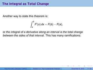
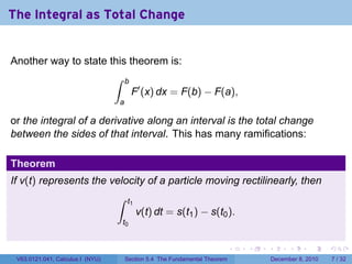
The Integral asTotal Change
Another way to state this theorem is:
∫ b
F′ (x) dx = F(b) − F(a),
a
or the integral of a derivative along an interval is the total change
between the sides of that interval. This has many ramifications:
. . . . . .
V63.0121.041, Calculus I (NYU) Section 5.4 The Fundamental Theorem December 8, 2010 7 / 32
8.
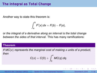
The Integral asTotal Change
Another way to state this theorem is:
∫ b
F′ (x) dx = F(b) − F(a),
a
or the integral of a derivative along an interval is the total change
between the sides of that interval. This has many ramifications:
Theorem
If v(t) represents the velocity of a particle moving rectilinearly, then
∫ t1
v(t) dt = s(t1 ) − s(t0 ).
t0
. . . . . .
V63.0121.041, Calculus I (NYU) Section 5.4 The Fundamental Theorem December 8, 2010 7 / 32
9.
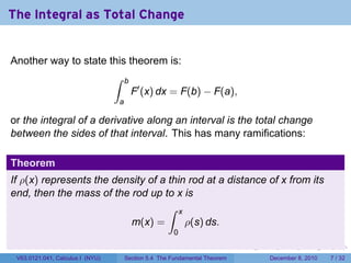
The Integral asTotal Change
Another way to state this theorem is:
∫ b
F′ (x) dx = F(b) − F(a),
a
or the integral of a derivative along an interval is the total change
between the sides of that interval. This has many ramifications:
Theorem
If MC(x) represents the marginal cost of making x units of a product,
then ∫ x
C(x) = C(0) + MC(q) dq.
0
. . . . . .
V63.0121.041, Calculus I (NYU) Section 5.4 The Fundamental Theorem December 8, 2010 7 / 32
10.
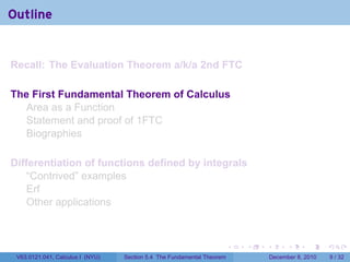
The Integral asTotal Change
Another way to state this theorem is:
∫ b
F′ (x) dx = F(b) − F(a),
a
or the integral of a derivative along an interval is the total change
between the sides of that interval. This has many ramifications:
Theorem
If ρ(x) represents the density of a thin rod at a distance of x from its
end, then the mass of the rod up to x is
∫ x
m(x) = ρ(s) ds.
0
. . . . . .
V63.0121.041, Calculus I (NYU) Section 5.4 The Fundamental Theorem December 8, 2010 7 / 32
11.
My first tableof integrals
.
∫ ∫ ∫
[f(x) + g(x)] dx = f(x) dx + g(x) dx
∫ ∫ ∫
xn+1
xn dx = + C (n ̸= −1) cf(x) dx = c f(x) dx
n+1 ∫
∫
1
ex dx = ex + C dx = ln |x| + C
x
∫ ∫
ax
sin x dx = − cos x + C ax dx = +C
ln a
∫ ∫
cos x dx = sin x + C csc2 x dx = − cot x + C
∫ ∫
2
sec x dx = tan x + C csc x cot x dx = − csc x + C
∫ ∫
1
sec x tan x dx = sec x + C √ dx = arcsin x + C
∫ 1 − x2
1
dx = arctan x + C
1 + x2
. . . . . .
V63.0121.041, Calculus I (NYU) Section 5.4 The Fundamental Theorem December 8, 2010 8 / 32
12.
Outline
Recall: The EvaluationTheorem a/k/a 2nd FTC
The First Fundamental Theorem of Calculus
Area as a Function
Statement and proof of 1FTC
Biographies
Differentiation of functions defined by integrals
“Contrived” examples
Erf
Other applications
. . . . . .
V63.0121.041, Calculus I (NYU) Section 5.4 The Fundamental Theorem December 8, 2010 9 / 32
13.
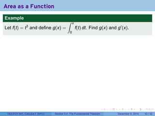
Area as aFunction
Example
∫ x
3
Let f(t) = t and define g(x) = f(t) dt. Find g(x) and g′ (x).
0
. . . . . .
V63.0121.041, Calculus I (NYU) Section 5.4 The Fundamental Theorem December 8, 2010 10 / 32
14.
Area as aFunction
Example
∫ x
3
Let f(t) = t and define g(x) = f(t) dt. Find g(x) and g′ (x).
0
Solution
Dividing the interval [0, x] into n pieces
x ix
gives ∆t = and ti = 0 + i∆t = .
n n
.
0 x
. . . . . .
V63.0121.041, Calculus I (NYU) Section 5.4 The Fundamental Theorem December 8, 2010 10 / 32
15.
Area as aFunction
Example
∫ x
3
Let f(t) = t and define g(x) = f(t) dt. Find g(x) and g′ (x).
0
Solution
Dividing the interval [0, x] into n pieces
x ix
gives ∆t = and ti = 0 + i∆t = . So
n n
.
0 x
. . . . . .
V63.0121.041, Calculus I (NYU) Section 5.4 The Fundamental Theorem December 8, 2010 10 / 32
16.
Area as aFunction
Example
∫ x
3
Let f(t) = t and define g(x) = f(t) dt. Find g(x) and g′ (x).
0
Solution
Dividing the interval [0, x] into n pieces
x ix
gives ∆t = and ti = 0 + i∆t = . So
n n
x x3 x (2x)3 x (nx)3
Rn = · 3+ · + ··· + ·
n n n n3 n n3
.
0 x
. . . . . .
V63.0121.041, Calculus I (NYU) Section 5.4 The Fundamental Theorem December 8, 2010 10 / 32
17.
Area as aFunction
Example
∫ x
3
Let f(t) = t and define g(x) = f(t) dt. Find g(x) and g′ (x).
0
Solution
Dividing the interval [0, x] into n pieces
x ix
gives ∆t = and ti = 0 + i∆t = . So
n n
x x3 x (2x)3 x (nx)3
Rn = · 3+ · + ··· + ·
n n n n3 n n3
x4 ( )
= 4 13 + 23 + 33 + · · · + n3
n
.
0 x
. . . . . .
V63.0121.041, Calculus I (NYU) Section 5.4 The Fundamental Theorem December 8, 2010 10 / 32
18.
Area as aFunction
Example
∫ x
3
Let f(t) = t and define g(x) = f(t) dt. Find g(x) and g′ (x).
0
Solution
Dividing the interval [0, x] into n pieces
x ix
gives ∆t = and ti = 0 + i∆t = . So
n n
x x3 x (2x)3 x (nx)3
Rn = · 3+ · + ··· + ·
n n n n3 n n3
x4 ( )
= 4 13 + 23 + 33 + · · · + n3
n
x4 [ ]2
.
0 x = 4 1 n(n + 1)
n 2
. . . . . .
V63.0121.041, Calculus I (NYU) Section 5.4 The Fundamental Theorem December 8, 2010 10 / 32
19.
Area as aFunction
Example
∫ x
3
Let f(t) = t and define g(x) = f(t) dt. Find g(x) and g′ (x).
0
Solution
Dividing the interval [0, x] into n pieces
x ix
gives ∆t = and ti = 0 + i∆t = . So
n n
x4 n2 (n + 1)2
Rn =
4n4
.
0 x
. . . . . .
V63.0121.041, Calculus I (NYU) Section 5.4 The Fundamental Theorem December 8, 2010 10 / 32
20.
Area as aFunction
Example
∫ x
3
Let f(t) = t and define g(x) = f(t) dt. Find g(x) and g′ (x).
0
Solution
Dividing the interval [0, x] into n pieces
x ix
gives ∆t = and ti = 0 + i∆t = . So
n n
x4 n2 (n + 1)2
Rn =
4n4
x4
So g(x) = lim Rn =
. x→∞ 4
0 x
. . . . . .
V63.0121.041, Calculus I (NYU) Section 5.4 The Fundamental Theorem December 8, 2010 10 / 32
21.
Area as aFunction
Example
∫ x
3
Let f(t) = t and define g(x) = f(t) dt. Find g(x) and g′ (x).
0
Solution
Dividing the interval [0, x] into n pieces
x ix
gives ∆t = and ti = 0 + i∆t = . So
n n
x4 n2 (n + 1)2
Rn =
4n4
x4
So g(x) = lim Rn = and g′ (x) = x3 .
. x→∞ 4
0 x
. . . . . .
V63.0121.041, Calculus I (NYU) Section 5.4 The Fundamental Theorem December 8, 2010 10 / 32
22.
The area functionin general
Let f be a function which is integrable (i.e., continuous or with finitely
many jump discontinuities) on [a, b]. Define
∫ x
g(x) = f(t) dt.
a
The variable is x; t is a “dummy” variable that’s integrated over.
Picture changing x and taking more of less of the region under the
curve.
Question: What does f tell you about g?
. . . . . .
V63.0121.041, Calculus I (NYU) Section 5.4 The Fundamental Theorem December 8, 2010 11 / 32
23.
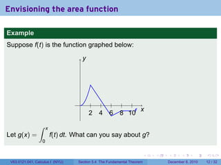
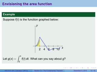
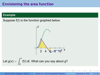
Envisioning the areafunction
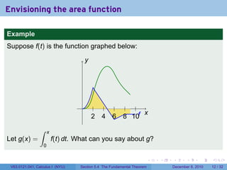
Example
Suppose f(t) is the function graphed below:
y
.
x
2 4 6 8 10f
∫ x
Let g(x) = f(t) dt. What can you say about g?
0
. . . . . .
V63.0121.041, Calculus I (NYU) Section 5.4 The Fundamental Theorem December 8, 2010 12 / 32
24.
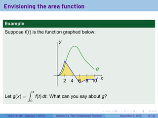
Envisioning the areafunction
Example
Suppose f(t) is the function graphed below:
y
g
.
x
2 4 6 8 10f
∫ x
Let g(x) = f(t) dt. What can you say about g?
0
. . . . . .
V63.0121.041, Calculus I (NYU) Section 5.4 The Fundamental Theorem December 8, 2010 12 / 32
25.
Envisioning the areafunction
Example
Suppose f(t) is the function graphed below:
y
g
.
x
2 4 6 8 10f
∫ x
Let g(x) = f(t) dt. What can you say about g?
0
. . . . . .
V63.0121.041, Calculus I (NYU) Section 5.4 The Fundamental Theorem December 8, 2010 12 / 32
26.
Envisioning the areafunction
Example
Suppose f(t) is the function graphed below:
y
g
.
x
2 4 6 8 10f
∫ x
Let g(x) = f(t) dt. What can you say about g?
0
. . . . . .
V63.0121.041, Calculus I (NYU) Section 5.4 The Fundamental Theorem December 8, 2010 12 / 32
27.
Envisioning the areafunction
Example
Suppose f(t) is the function graphed below:
y
g
.
x
2 4 6 8 10f
∫ x
Let g(x) = f(t) dt. What can you say about g?
0
. . . . . .
V63.0121.041, Calculus I (NYU) Section 5.4 The Fundamental Theorem December 8, 2010 12 / 32
28.
Envisioning the areafunction
Example
Suppose f(t) is the function graphed below:
y
g
.
x
2 4 6 8 10f
∫ x
Let g(x) = f(t) dt. What can you say about g?
0
. . . . . .
V63.0121.041, Calculus I (NYU) Section 5.4 The Fundamental Theorem December 8, 2010 12 / 32
29.
Envisioning the areafunction
Example
Suppose f(t) is the function graphed below:
y
g
.
x
2 4 6 8 10f
∫ x
Let g(x) = f(t) dt. What can you say about g?
0
. . . . . .
V63.0121.041, Calculus I (NYU) Section 5.4 The Fundamental Theorem December 8, 2010 12 / 32
30.
Envisioning the areafunction
Example
Suppose f(t) is the function graphed below:
y
g
.
x
2 4 6 8 10f
∫ x
Let g(x) = f(t) dt. What can you say about g?
0
. . . . . .
V63.0121.041, Calculus I (NYU) Section 5.4 The Fundamental Theorem December 8, 2010 12 / 32
31.
Envisioning the areafunction
Example
Suppose f(t) is the function graphed below:
y
g
.
x
2 4 6 8 10f
∫ x
Let g(x) = f(t) dt. What can you say about g?
0
. . . . . .
V63.0121.041, Calculus I (NYU) Section 5.4 The Fundamental Theorem December 8, 2010 12 / 32
32.
Envisioning the areafunction
Example
Suppose f(t) is the function graphed below:
y
g
.
x
2 4 6 8 10f
∫ x
Let g(x) = f(t) dt. What can you say about g?
0
. . . . . .
V63.0121.041, Calculus I (NYU) Section 5.4 The Fundamental Theorem December 8, 2010 12 / 32
33.
Envisioning the areafunction
Example
Suppose f(t) is the function graphed below:
y
g
.
x
2 4 6 8 10f
∫ x
Let g(x) = f(t) dt. What can you say about g?
0
. . . . . .
V63.0121.041, Calculus I (NYU) Section 5.4 The Fundamental Theorem December 8, 2010 12 / 32
34.
Envisioning the areafunction
Example
Suppose f(t) is the function graphed below:
y
g
.
x
2 4 6 8 10f
∫ x
Let g(x) = f(t) dt. What can you say about g?
0
. . . . . .
V63.0121.041, Calculus I (NYU) Section 5.4 The Fundamental Theorem December 8, 2010 12 / 32
35.
features of gfrom f
y
Interval sign monotonicity monotonicity concavity
of f of g of f of g
g
. [0, 2] + ↗ ↗ ⌣
fx
2 4 6 8 10 [2, 4.5] + ↗ ↘ ⌢
[4.5, 6] − ↘ ↘ ⌢
[6, 8] − ↘ ↗ ⌣
[8, 10] − ↘ → none
. . . . . .
V63.0121.041, Calculus I (NYU) Section 5.4 The Fundamental Theorem December 8, 2010 13 / 32
36.
features of gfrom f
y
Interval sign monotonicity monotonicity concavity
of f of g of f of g
g
. [0, 2] + ↗ ↗ ⌣
fx
2 4 6 8 10 [2, 4.5] + ↗ ↘ ⌢
[4.5, 6] − ↘ ↘ ⌢
[6, 8] − ↘ ↗ ⌣
[8, 10] − ↘ → none
We see that g is behaving a lot like an antiderivative of f.
. . . . . .
V63.0121.041, Calculus I (NYU) Section 5.4 The Fundamental Theorem December 8, 2010 13 / 32
37.
Another Big TimeTheorem
Theorem (The First Fundamental Theorem of Calculus)
Let f be an integrable function on [a, b] and define
∫ x
g(x) = f(t) dt.
a
If f is continuous at x in (a, b), then g is differentiable at x and
g′ (x) = f(x).
. . . . . .
V63.0121.041, Calculus I (NYU) Section 5.4 The Fundamental Theorem December 8, 2010 14 / 32
38.
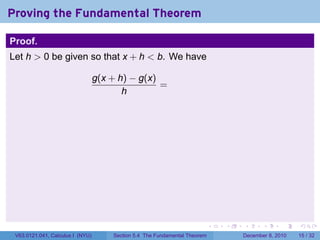
Proving the FundamentalTheorem
Proof.
Let h > 0 be given so that x + h < b. We have
g(x + h) − g(x)
=
h
. . . . . .
V63.0121.041, Calculus I (NYU) Section 5.4 The Fundamental Theorem December 8, 2010 15 / 32
39.
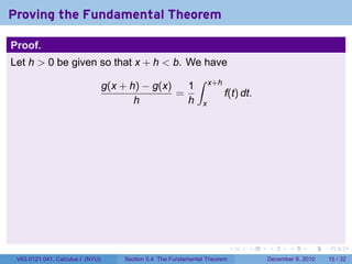
Proving the FundamentalTheorem
Proof.
Let h > 0 be given so that x + h < b. We have
∫
g(x + h) − g(x) 1 x+h
= f(t) dt.
h h x
. . . . . .
V63.0121.041, Calculus I (NYU) Section 5.4 The Fundamental Theorem December 8, 2010 15 / 32
40.
Proving the FundamentalTheorem
Proof.
Let h > 0 be given so that x + h < b. We have
∫
g(x + h) − g(x) 1 x+h
= f(t) dt.
h h x
Let Mh be the maximum value of f on [x, x + h], and let mh the minimum
value of f on [x, x + h]. From §5.2 we have
∫ x+h
f(t) dt
x
. . . . . .
V63.0121.041, Calculus I (NYU) Section 5.4 The Fundamental Theorem December 8, 2010 15 / 32
41.
Proving the FundamentalTheorem
Proof.
Let h > 0 be given so that x + h < b. We have
∫
g(x + h) − g(x) 1 x+h
= f(t) dt.
h h x
Let Mh be the maximum value of f on [x, x + h], and let mh the minimum
value of f on [x, x + h]. From §5.2 we have
∫ x+h
f(t) dt ≤ Mh · h
x
. . . . . .
V63.0121.041, Calculus I (NYU) Section 5.4 The Fundamental Theorem December 8, 2010 15 / 32
42.
Proving the FundamentalTheorem
Proof.
Let h > 0 be given so that x + h < b. We have
∫
g(x + h) − g(x) 1 x+h
= f(t) dt.
h h x
Let Mh be the maximum value of f on [x, x + h], and let mh the minimum
value of f on [x, x + h]. From §5.2 we have
∫ x+h
mh · h ≤ f(t) dt ≤ Mh · h
x
. . . . . .
V63.0121.041, Calculus I (NYU) Section 5.4 The Fundamental Theorem December 8, 2010 15 / 32
43.
Proving the FundamentalTheorem
Proof.
Let h > 0 be given so that x + h < b. We have
∫
g(x + h) − g(x) 1 x+h
= f(t) dt.
h h x
Let Mh be the maximum value of f on [x, x + h], and let mh the minimum
value of f on [x, x + h]. From §5.2 we have
∫ x+h
mh · h ≤ f(t) dt ≤ Mh · h
x
So
g(x + h) − g(x)
mh ≤ ≤ Mh .
h
. . . . . .
V63.0121.041, Calculus I (NYU) Section 5.4 The Fundamental Theorem December 8, 2010 15 / 32
44.
Proving the FundamentalTheorem
Proof.
Let h > 0 be given so that x + h < b. We have
∫
g(x + h) − g(x) 1 x+h
= f(t) dt.
h h x
Let Mh be the maximum value of f on [x, x + h], and let mh the minimum
value of f on [x, x + h]. From §5.2 we have
∫ x+h
mh · h ≤ f(t) dt ≤ Mh · h
x
So
g(x + h) − g(x)
mh ≤ ≤ Mh .
h
As h → 0, both mh and Mh tend to f(x).
. . . . . .
V63.0121.041, Calculus I (NYU) Section 5.4 The Fundamental Theorem December 8, 2010 15 / 32
45.
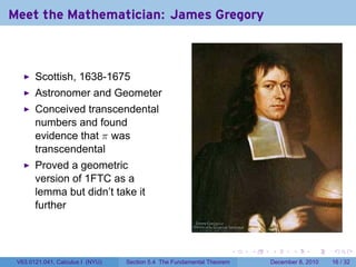
Meet the Mathematician:James Gregory
Scottish, 1638-1675
Astronomer and Geometer
Conceived transcendental
numbers and found
evidence that π was
transcendental
Proved a geometric
version of 1FTC as a
lemma but didn’t take it
further
. . . . . .
V63.0121.041, Calculus I (NYU) Section 5.4 The Fundamental Theorem December 8, 2010 16 / 32
46.
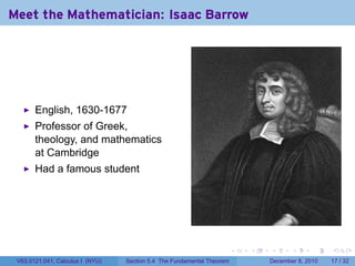
Meet the Mathematician:Isaac Barrow
English, 1630-1677
Professor of Greek,
theology, and mathematics
at Cambridge
Had a famous student
. . . . . .
V63.0121.041, Calculus I (NYU) Section 5.4 The Fundamental Theorem December 8, 2010 17 / 32
47.
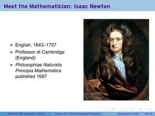
Meet the Mathematician:Isaac Newton
English, 1643–1727
Professor at Cambridge
(England)
Philosophiae Naturalis
Principia Mathematica
published 1687
. . . . . .
V63.0121.041, Calculus I (NYU) Section 5.4 The Fundamental Theorem December 8, 2010 18 / 32
48.
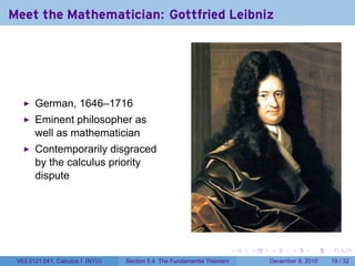
Meet the Mathematician:Gottfried Leibniz
German, 1646–1716
Eminent philosopher as
well as mathematician
Contemporarily disgraced
by the calculus priority
dispute
. . . . . .
V63.0121.041, Calculus I (NYU) Section 5.4 The Fundamental Theorem December 8, 2010 19 / 32
49.
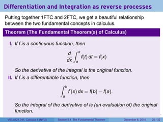
Differentiation and Integrationas reverse processes
Putting together 1FTC and 2FTC, we get a beautiful relationship
between the two fundamental concepts in calculus.
Theorem (The Fundamental Theorem(s) of Calculus)
I. If f is a continuous function, then
∫ x
d
f(t) dt = f(x)
dx a
So the derivative of the integral is the original function.
II. If f is a differentiable function, then
∫ b
f′ (x) dx = f(b) − f(a).
a
So the integral of the derivative of is (an evaluation of) the original
function.
. . . . . .
V63.0121.041, Calculus I (NYU) Section 5.4 The Fundamental Theorem December 8, 2010 20 / 32
50.
Outline
Recall: The EvaluationTheorem a/k/a 2nd FTC
The First Fundamental Theorem of Calculus
Area as a Function
Statement and proof of 1FTC
Biographies
Differentiation of functions defined by integrals
“Contrived” examples
Erf
Other applications
. . . . . .
V63.0121.041, Calculus I (NYU) Section 5.4 The Fundamental Theorem December 8, 2010 21 / 32
51.
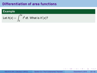
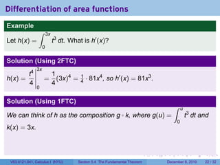
Differentiation of areafunctions
Example
∫ 3x
Let h(x) = t3 dt. What is h′ (x)?
0
. . . . . .
V63.0121.041, Calculus I (NYU) Section 5.4 The Fundamental Theorem December 8, 2010 22 / 32
52.
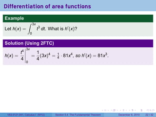
Differentiation of areafunctions
Example
∫ 3x
Let h(x) = t3 dt. What is h′ (x)?
0
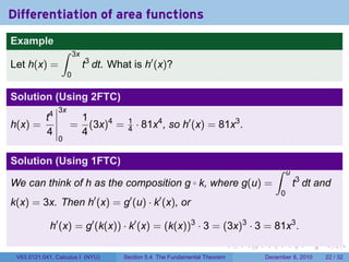
Solution (Using 2FTC)
3x
t4 1
h(x) = = (3x)4 = 1
4 · 81x4 , so h′ (x) = 81x3 .
4 4
0
. . . . . .
V63.0121.041, Calculus I (NYU) Section 5.4 The Fundamental Theorem December 8, 2010 22 / 32
53.
Differentiation of areafunctions
Example
∫ 3x
Let h(x) = t3 dt. What is h′ (x)?
0
Solution (Using 2FTC)
3x
t4 1
h(x) = = (3x)4 = 1
4 · 81x4 , so h′ (x) = 81x3 .
4 4
0
Solution (Using 1FTC)
∫ u
We can think of h as the composition g k, where g(u) = ◦ t3 dt and
0
k(x) = 3x.
. . . . . .
V63.0121.041, Calculus I (NYU) Section 5.4 The Fundamental Theorem December 8, 2010 22 / 32
54.
Differentiation of areafunctions
Example
∫ 3x
Let h(x) = t3 dt. What is h′ (x)?
0
Solution (Using 2FTC)
3x
t4 1
h(x) = = (3x)4 = 1
4 · 81x4 , so h′ (x) = 81x3 .
4 4
0
Solution (Using 1FTC)
∫ u
We can think of h as the composition g k, where g(u) = ◦ t3 dt and
0
k(x) = 3x. Then h′ (x) = g′ (u) · k′ (x), or
h′ (x) = g′ (k(x)) · k′ (x) = (k(x))3 · 3 = (3x)3 · 3 = 81x3 .
. . . . . .
V63.0121.041, Calculus I (NYU) Section 5.4 The Fundamental Theorem December 8, 2010 22 / 32
55.
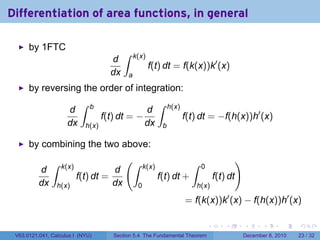
Differentiation of areafunctions, in general
by 1FTC
∫ k(x)
d
f(t) dt = f(k(x))k′ (x)
dx a
by reversing the order of integration:
∫ b ∫ h(x)
d d
f(t) dt = − f(t) dt = −f(h(x))h′ (x)
dx h(x) dx b
by combining the two above:
∫ (∫ ∫ )
k(x) k(x) 0
d d
f(t) dt = f(t) dt + f(t) dt
dx h(x) dx 0 h(x)
= f(k(x))k′ (x) − f(h(x))h′ (x)
. . . . . .
V63.0121.041, Calculus I (NYU) Section 5.4 The Fundamental Theorem December 8, 2010 23 / 32
56.
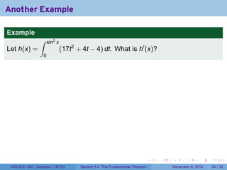
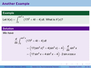
Another Example
Example
∫ sin2 x
Let h(x) = (17t2 + 4t − 4) dt. What is h′ (x)?
0
. . . . . .
V63.0121.041, Calculus I (NYU) Section 5.4 The Fundamental Theorem December 8, 2010 24 / 32
57.
Another Example
Example
∫ sin2 x
Let h(x) = (17t2 + 4t − 4) dt. What is h′ (x)?
0
Solution
We have
∫ sin2 x
d
(17t2 + 4t − 4) dt
dx 0
( d )
2 2
= 17(sin x) + 4(sin x) − 4 ·
2
sin2 x
( ) dx
= 17 sin4 x + 4 sin2 x − 4 · 2 sin x cos x
. . . . . .
V63.0121.041, Calculus I (NYU) Section 5.4 The Fundamental Theorem December 8, 2010 24 / 32
58.
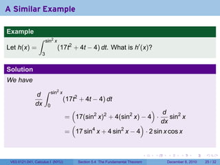
A Similar Example
Example
∫ sin2 x
Let h(x) = (17t2 + 4t − 4) dt. What is h′ (x)?
3
. . . . . .
V63.0121.041, Calculus I (NYU) Section 5.4 The Fundamental Theorem December 8, 2010 25 / 32
59.
A Similar Example
Example
∫ sin2 x
Let h(x) = (17t2 + 4t − 4) dt. What is h′ (x)?
3
Solution
We have
∫ sin2 x
d
(17t2 + 4t − 4) dt
dx 0
( d )
2 2
= 17(sin x) + 4(sin x) − 4 ·
2
sin2 x
( ) dx
= 17 sin4 x + 4 sin2 x − 4 · 2 sin x cos x
. . . . . .
V63.0121.041, Calculus I (NYU) Section 5.4 The Fundamental Theorem December 8, 2010 25 / 32
60.
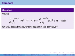
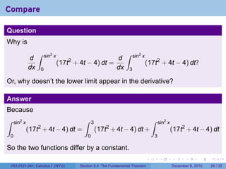
Compare
Question
Why is
∫ sin2 x ∫ sin2 x
d d
(17t + 4t − 4) dt =
2
(17t2 + 4t − 4) dt?
dx 0 dx 3
Or, why doesn’t the lower limit appear in the derivative?
. . . . . .
V63.0121.041, Calculus I (NYU) Section 5.4 The Fundamental Theorem December 8, 2010 26 / 32
61.
Compare
Question
Why is
∫ sin2 x ∫ sin2 x
d d
(17t + 4t − 4) dt =
2
(17t2 + 4t − 4) dt?
dx 0 dx 3
Or, why doesn’t the lower limit appear in the derivative?
Answer
Because
∫ sin2 x ∫ 3 ∫ sin2 x
(17t2 + 4t − 4) dt = (17t2 + 4t − 4) dt + (17t2 + 4t − 4) dt
0 0 3
So the two functions differ by a constant.
. . . . . .
V63.0121.041, Calculus I (NYU) Section 5.4 The Fundamental Theorem December 8, 2010 26 / 32
62.
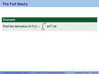
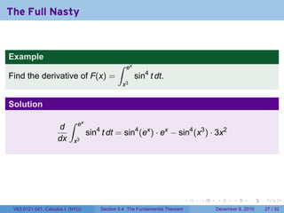
The Full Nasty
Example
∫ ex
Find the derivative of F(x) = sin4 t dt.
x3
. . . . . .
V63.0121.041, Calculus I (NYU) Section 5.4 The Fundamental Theorem December 8, 2010 27 / 32
63.
The Full Nasty
Example
∫ ex
Find the derivative of F(x) = sin4 t dt.
x3
Solution
∫ ex
d
sin4 t dt = sin4 (ex ) · ex − sin4 (x3 ) · 3x2
dx x3
. . . . . .
V63.0121.041, Calculus I (NYU) Section 5.4 The Fundamental Theorem December 8, 2010 27 / 32
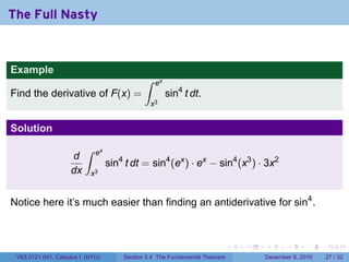
64.
The Full Nasty
Example
∫ ex
Find the derivative of F(x) = sin4 t dt.
x3
Solution
∫ ex
d
sin4 t dt = sin4 (ex ) · ex − sin4 (x3 ) · 3x2
dx x3
Notice here it’s much easier than finding an antiderivative for sin4 .
. . . . . .
V63.0121.041, Calculus I (NYU) Section 5.4 The Fundamental Theorem December 8, 2010 27 / 32
65.
Why use 1FTC?
Question
Whywould we use 1FTC to find the derivative of an integral? It seems
like confusion for its own sake.
. . . . . .
V63.0121.041, Calculus I (NYU) Section 5.4 The Fundamental Theorem December 8, 2010 28 / 32
66.
Why use 1FTC?
Question
Whywould we use 1FTC to find the derivative of an integral? It seems
like confusion for its own sake.
Answer
Some functions are difficult or impossible to integrate in
elementary terms.
. . . . . .
V63.0121.041, Calculus I (NYU) Section 5.4 The Fundamental Theorem December 8, 2010 28 / 32
67.
Why use 1FTC?
Question
Whywould we use 1FTC to find the derivative of an integral? It seems
like confusion for its own sake.
Answer
Some functions are difficult or impossible to integrate in
elementary terms.
Some functions are naturally defined in terms of other integrals.
. . . . . .
V63.0121.041, Calculus I (NYU) Section 5.4 The Fundamental Theorem December 8, 2010 28 / 32
68.
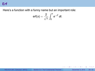
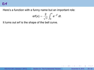
Erf
Here’s a functionwith a funny name but an important role:
∫ x
2
e−t dt.
2
erf(x) = √
π 0
. . . . . .
V63.0121.041, Calculus I (NYU) Section 5.4 The Fundamental Theorem December 8, 2010 29 / 32
69.
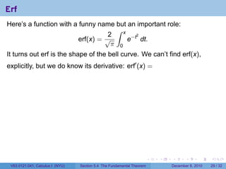
Erf
Here’s a functionwith a funny name but an important role:
∫ x
2
e−t dt.
2
erf(x) = √
π 0
It turns out erf is the shape of the bell curve.
. . . . . .
V63.0121.041, Calculus I (NYU) Section 5.4 The Fundamental Theorem December 8, 2010 29 / 32
70.
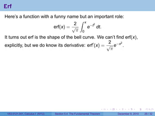
Erf
Here’s a functionwith a funny name but an important role:
∫ x
2
e−t dt.
2
erf(x) = √
π 0
It turns out erf is the shape of the bell curve. We can’t find erf(x),
explicitly, but we do know its derivative: erf′ (x) =
. . . . . .
V63.0121.041, Calculus I (NYU) Section 5.4 The Fundamental Theorem December 8, 2010 29 / 32
71.
Erf
Here’s a functionwith a funny name but an important role:
∫ x
2
e−t dt.
2
erf(x) = √
π 0
It turns out erf is the shape of the bell curve. We can’t find erf(x),
2
explicitly, but we do know its derivative: erf′ (x) = √ e−x .
2
π
. . . . . .
V63.0121.041, Calculus I (NYU) Section 5.4 The Fundamental Theorem December 8, 2010 29 / 32
72.
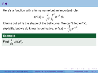
Erf
Here’s a functionwith a funny name but an important role:
∫ x
2
e−t dt.
2
erf(x) = √
π 0
It turns out erf is the shape of the bell curve. We can’t find erf(x),
2
explicitly, but we do know its derivative: erf′ (x) = √ e−x .
2
π
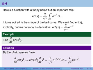
Example
d
Find erf(x2 ).
dx
. . . . . .
V63.0121.041, Calculus I (NYU) Section 5.4 The Fundamental Theorem December 8, 2010 29 / 32
73.
Erf
Here’s a functionwith a funny name but an important role:
∫ x
2
e−t dt.
2
erf(x) = √
π 0
It turns out erf is the shape of the bell curve. We can’t find erf(x),
2
explicitly, but we do know its derivative: erf′ (x) = √ e−x .
2
π
Example
d
Find erf(x2 ).
dx
Solution
By the chain rule we have
d d 2 4
erf(x2 ) = erf′ (x2 ) x2 = √ e−(x ) 2x = √ xe−x .
2 2 4
dx dx π π
. . . . . .
V63.0121.041, Calculus I (NYU) Section 5.4 The Fundamental Theorem December 8, 2010 29 / 32
74.
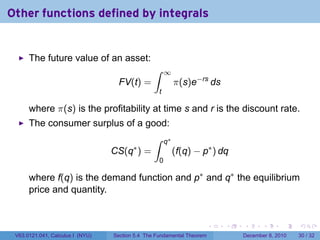
Other functions definedby integrals
The future value of an asset:
∫ ∞
FV(t) = π(s)e−rs ds
t
where π(s) is the profitability at time s and r is the discount rate.
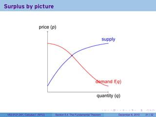
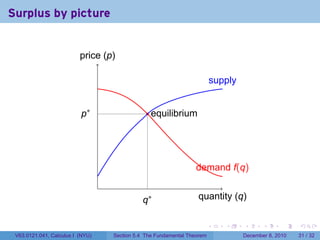
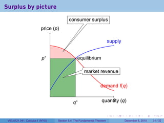
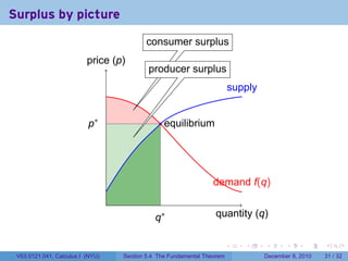
The consumer surplus of a good:
∫ q∗
∗
CS(q ) = (f(q) − p∗ ) dq
0
where f(q) is the demand function and p∗ and q∗ the equilibrium
price and quantity.
. . . . . .
V63.0121.041, Calculus I (NYU) Section 5.4 The Fundamental Theorem December 8, 2010 30 / 32
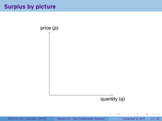
75.
Surplus by picture
price (p)
.
quantity (q)
. . . . . .
V63.0121.041, Calculus I (NYU) Section 5.4 The Fundamental Theorem December 8, 2010 31 / 32
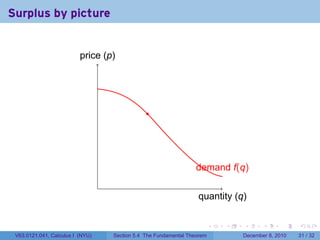
76.
Surplus by picture
price (p)
demand f(q)
.
quantity (q)
. . . . . .
V63.0121.041, Calculus I (NYU) Section 5.4 The Fundamental Theorem December 8, 2010 31 / 32
77.
Surplus by picture
price (p)
supply
demand f(q)
.
quantity (q)
. . . . . .
V63.0121.041, Calculus I (NYU) Section 5.4 The Fundamental Theorem December 8, 2010 31 / 32
78.
Surplus by picture
price (p)
supply
p∗ equilibrium
demand f(q)
.
q∗ quantity (q)
. . . . . .
V63.0121.041, Calculus I (NYU) Section 5.4 The Fundamental Theorem December 8, 2010 31 / 32
79.
Surplus by picture
price (p)
supply
p∗ equilibrium
market revenue
demand f(q)
.
q∗ quantity (q)
. . . . . .
V63.0121.041, Calculus I (NYU) Section 5.4 The Fundamental Theorem December 8, 2010 31 / 32
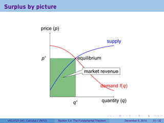
80.
Surplus by picture
consumer surplus
price (p)
supply
p∗ equilibrium
market revenue
demand f(q)
.
q∗ quantity (q)
. . . . . .
V63.0121.041, Calculus I (NYU) Section 5.4 The Fundamental Theorem December 8, 2010 31 / 32
81.
Surplus by picture
consumer surplus
price (p)
producer surplus
supply
p∗ equilibrium
demand f(q)
.
q∗ quantity (q)
. . . . . .
V63.0121.041, Calculus I (NYU) Section 5.4 The Fundamental Theorem December 8, 2010 31 / 32
82.
Summary
Functions defined as integrals can be differentiated using the first
FTC: ∫ x
d
f(t) dt = f(x)
dx a
The two FTCs link the two major processes in calculus:
differentiation and integration
∫
F′ (x) dx = F(x) + C
Follow the calculus wars on twitter: #calcwars
. . . . . .
V63.0121.041, Calculus I (NYU) Section 5.4 The Fundamental Theorem December 8, 2010 32 / 32

![The definite integral as a limit
Definition
If f is a function defined on [a, b], the definite integral of f from a to b
is the number ∫ b ∑n
f(x) dx = lim f(ci ) ∆x
a ∆x→0
i=1
. . . . . .
V63.0121.041, Calculus I (NYU) Section 5.4 The Fundamental Theorem December 8, 2010 5 / 32](https://image.slidesharecdn.com/lesson26-thefundamentaltheoremofcalculus041slides-101208151253-phpapp02/85/Lesson-26-The-Fundamental-Theorem-of-Calculus-Section-041-slides-5-320.jpg)
![Big time Theorem
Theorem (The Second Fundamental Theorem of Calculus)
Suppose f is integrable on [a, b] and f = F′ for another function F, then
∫ b
f(x) dx = F(b) − F(a).
a
. . . . . .
V63.0121.041, Calculus I (NYU) Section 5.4 The Fundamental Theorem December 8, 2010 6 / 32](https://image.slidesharecdn.com/lesson26-thefundamentaltheoremofcalculus041slides-101208151253-phpapp02/85/Lesson-26-The-Fundamental-Theorem-of-Calculus-Section-041-slides-6-320.jpg)
![My first table of integrals
.
∫ ∫ ∫
[f(x) + g(x)] dx = f(x) dx + g(x) dx
∫ ∫ ∫
xn+1
xn dx = + C (n ̸= −1) cf(x) dx = c f(x) dx
n+1 ∫
∫
1
ex dx = ex + C dx = ln |x| + C
x
∫ ∫
ax
sin x dx = − cos x + C ax dx = +C
ln a
∫ ∫
cos x dx = sin x + C csc2 x dx = − cot x + C
∫ ∫
2
sec x dx = tan x + C csc x cot x dx = − csc x + C
∫ ∫
1
sec x tan x dx = sec x + C √ dx = arcsin x + C
∫ 1 − x2
1
dx = arctan x + C
1 + x2
. . . . . .
V63.0121.041, Calculus I (NYU) Section 5.4 The Fundamental Theorem December 8, 2010 8 / 32](https://image.slidesharecdn.com/lesson26-thefundamentaltheoremofcalculus041slides-101208151253-phpapp02/85/Lesson-26-The-Fundamental-Theorem-of-Calculus-Section-041-slides-11-320.jpg)
![Area as a Function
Example
∫ x
3
Let f(t) = t and define g(x) = f(t) dt. Find g(x) and g′ (x).
0
Solution
Dividing the interval [0, x] into n pieces
x ix
gives ∆t = and ti = 0 + i∆t = .
n n
.
0 x
. . . . . .
V63.0121.041, Calculus I (NYU) Section 5.4 The Fundamental Theorem December 8, 2010 10 / 32](https://image.slidesharecdn.com/lesson26-thefundamentaltheoremofcalculus041slides-101208151253-phpapp02/85/Lesson-26-The-Fundamental-Theorem-of-Calculus-Section-041-slides-14-320.jpg)
![Area as a Function
Example
∫ x
3
Let f(t) = t and define g(x) = f(t) dt. Find g(x) and g′ (x).
0
Solution
Dividing the interval [0, x] into n pieces
x ix
gives ∆t = and ti = 0 + i∆t = . So
n n
.
0 x
. . . . . .
V63.0121.041, Calculus I (NYU) Section 5.4 The Fundamental Theorem December 8, 2010 10 / 32](https://image.slidesharecdn.com/lesson26-thefundamentaltheoremofcalculus041slides-101208151253-phpapp02/85/Lesson-26-The-Fundamental-Theorem-of-Calculus-Section-041-slides-15-320.jpg)
![Area as a Function
Example
∫ x
3
Let f(t) = t and define g(x) = f(t) dt. Find g(x) and g′ (x).
0
Solution
Dividing the interval [0, x] into n pieces
x ix
gives ∆t = and ti = 0 + i∆t = . So
n n
x x3 x (2x)3 x (nx)3
Rn = · 3+ · + ··· + ·
n n n n3 n n3
.
0 x
. . . . . .
V63.0121.041, Calculus I (NYU) Section 5.4 The Fundamental Theorem December 8, 2010 10 / 32](https://image.slidesharecdn.com/lesson26-thefundamentaltheoremofcalculus041slides-101208151253-phpapp02/85/Lesson-26-The-Fundamental-Theorem-of-Calculus-Section-041-slides-16-320.jpg)
![Area as a Function
Example
∫ x
3
Let f(t) = t and define g(x) = f(t) dt. Find g(x) and g′ (x).
0
Solution
Dividing the interval [0, x] into n pieces
x ix
gives ∆t = and ti = 0 + i∆t = . So
n n
x x3 x (2x)3 x (nx)3
Rn = · 3+ · + ··· + ·
n n n n3 n n3
x4 ( )
= 4 13 + 23 + 33 + · · · + n3
n
.
0 x
. . . . . .
V63.0121.041, Calculus I (NYU) Section 5.4 The Fundamental Theorem December 8, 2010 10 / 32](https://image.slidesharecdn.com/lesson26-thefundamentaltheoremofcalculus041slides-101208151253-phpapp02/85/Lesson-26-The-Fundamental-Theorem-of-Calculus-Section-041-slides-17-320.jpg)
![Area as a Function
Example
∫ x
3
Let f(t) = t and define g(x) = f(t) dt. Find g(x) and g′ (x).
0
Solution
Dividing the interval [0, x] into n pieces
x ix
gives ∆t = and ti = 0 + i∆t = . So
n n
x x3 x (2x)3 x (nx)3
Rn = · 3+ · + ··· + ·
n n n n3 n n3
x4 ( )
= 4 13 + 23 + 33 + · · · + n3
n
x4 [ ]2
.
0 x = 4 1 n(n + 1)
n 2
. . . . . .
V63.0121.041, Calculus I (NYU) Section 5.4 The Fundamental Theorem December 8, 2010 10 / 32](https://image.slidesharecdn.com/lesson26-thefundamentaltheoremofcalculus041slides-101208151253-phpapp02/85/Lesson-26-The-Fundamental-Theorem-of-Calculus-Section-041-slides-18-320.jpg)
![Area as a Function
Example
∫ x
3
Let f(t) = t and define g(x) = f(t) dt. Find g(x) and g′ (x).
0
Solution
Dividing the interval [0, x] into n pieces
x ix
gives ∆t = and ti = 0 + i∆t = . So
n n
x4 n2 (n + 1)2
Rn =
4n4
.
0 x
. . . . . .
V63.0121.041, Calculus I (NYU) Section 5.4 The Fundamental Theorem December 8, 2010 10 / 32](https://image.slidesharecdn.com/lesson26-thefundamentaltheoremofcalculus041slides-101208151253-phpapp02/85/Lesson-26-The-Fundamental-Theorem-of-Calculus-Section-041-slides-19-320.jpg)
![Area as a Function
Example
∫ x
3
Let f(t) = t and define g(x) = f(t) dt. Find g(x) and g′ (x).
0
Solution
Dividing the interval [0, x] into n pieces
x ix
gives ∆t = and ti = 0 + i∆t = . So
n n
x4 n2 (n + 1)2
Rn =
4n4
x4
So g(x) = lim Rn =
. x→∞ 4
0 x
. . . . . .
V63.0121.041, Calculus I (NYU) Section 5.4 The Fundamental Theorem December 8, 2010 10 / 32](https://image.slidesharecdn.com/lesson26-thefundamentaltheoremofcalculus041slides-101208151253-phpapp02/85/Lesson-26-The-Fundamental-Theorem-of-Calculus-Section-041-slides-20-320.jpg)
![Area as a Function
Example
∫ x
3
Let f(t) = t and define g(x) = f(t) dt. Find g(x) and g′ (x).
0
Solution
Dividing the interval [0, x] into n pieces
x ix
gives ∆t = and ti = 0 + i∆t = . So
n n
x4 n2 (n + 1)2
Rn =
4n4
x4
So g(x) = lim Rn = and g′ (x) = x3 .
. x→∞ 4
0 x
. . . . . .
V63.0121.041, Calculus I (NYU) Section 5.4 The Fundamental Theorem December 8, 2010 10 / 32](https://image.slidesharecdn.com/lesson26-thefundamentaltheoremofcalculus041slides-101208151253-phpapp02/85/Lesson-26-The-Fundamental-Theorem-of-Calculus-Section-041-slides-21-320.jpg)
![The area function in general
Let f be a function which is integrable (i.e., continuous or with finitely
many jump discontinuities) on [a, b]. Define
∫ x
g(x) = f(t) dt.
a
The variable is x; t is a “dummy” variable that’s integrated over.
Picture changing x and taking more of less of the region under the
curve.
Question: What does f tell you about g?
. . . . . .
V63.0121.041, Calculus I (NYU) Section 5.4 The Fundamental Theorem December 8, 2010 11 / 32](https://image.slidesharecdn.com/lesson26-thefundamentaltheoremofcalculus041slides-101208151253-phpapp02/85/Lesson-26-The-Fundamental-Theorem-of-Calculus-Section-041-slides-22-320.jpg)


![features of g from f
y
Interval sign monotonicity monotonicity concavity
of f of g of f of g
g
. [0, 2] + ↗ ↗ ⌣
fx
2 4 6 8 10 [2, 4.5] + ↗ ↘ ⌢
[4.5, 6] − ↘ ↘ ⌢
[6, 8] − ↘ ↗ ⌣
[8, 10] − ↘ → none
. . . . . .
V63.0121.041, Calculus I (NYU) Section 5.4 The Fundamental Theorem December 8, 2010 13 / 32](https://image.slidesharecdn.com/lesson26-thefundamentaltheoremofcalculus041slides-101208151253-phpapp02/85/Lesson-26-The-Fundamental-Theorem-of-Calculus-Section-041-slides-35-320.jpg)
![features of g from f
y
Interval sign monotonicity monotonicity concavity
of f of g of f of g
g
. [0, 2] + ↗ ↗ ⌣
fx
2 4 6 8 10 [2, 4.5] + ↗ ↘ ⌢
[4.5, 6] − ↘ ↘ ⌢
[6, 8] − ↘ ↗ ⌣
[8, 10] − ↘ → none
We see that g is behaving a lot like an antiderivative of f.
. . . . . .
V63.0121.041, Calculus I (NYU) Section 5.4 The Fundamental Theorem December 8, 2010 13 / 32](https://image.slidesharecdn.com/lesson26-thefundamentaltheoremofcalculus041slides-101208151253-phpapp02/85/Lesson-26-The-Fundamental-Theorem-of-Calculus-Section-041-slides-36-320.jpg)
![Another Big Time Theorem
Theorem (The First Fundamental Theorem of Calculus)
Let f be an integrable function on [a, b] and define
∫ x
g(x) = f(t) dt.
a
If f is continuous at x in (a, b), then g is differentiable at x and
g′ (x) = f(x).
. . . . . .
V63.0121.041, Calculus I (NYU) Section 5.4 The Fundamental Theorem December 8, 2010 14 / 32](https://image.slidesharecdn.com/lesson26-thefundamentaltheoremofcalculus041slides-101208151253-phpapp02/85/Lesson-26-The-Fundamental-Theorem-of-Calculus-Section-041-slides-37-320.jpg)
![Proving the Fundamental Theorem
Proof.
Let h > 0 be given so that x + h < b. We have
∫
g(x + h) − g(x) 1 x+h
= f(t) dt.
h h x
Let Mh be the maximum value of f on [x, x + h], and let mh the minimum
value of f on [x, x + h]. From §5.2 we have
∫ x+h
f(t) dt
x
. . . . . .
V63.0121.041, Calculus I (NYU) Section 5.4 The Fundamental Theorem December 8, 2010 15 / 32](https://image.slidesharecdn.com/lesson26-thefundamentaltheoremofcalculus041slides-101208151253-phpapp02/85/Lesson-26-The-Fundamental-Theorem-of-Calculus-Section-041-slides-40-320.jpg)
![Proving the Fundamental Theorem
Proof.
Let h > 0 be given so that x + h < b. We have
∫
g(x + h) − g(x) 1 x+h
= f(t) dt.
h h x
Let Mh be the maximum value of f on [x, x + h], and let mh the minimum
value of f on [x, x + h]. From §5.2 we have
∫ x+h
f(t) dt ≤ Mh · h
x
. . . . . .
V63.0121.041, Calculus I (NYU) Section 5.4 The Fundamental Theorem December 8, 2010 15 / 32](https://image.slidesharecdn.com/lesson26-thefundamentaltheoremofcalculus041slides-101208151253-phpapp02/85/Lesson-26-The-Fundamental-Theorem-of-Calculus-Section-041-slides-41-320.jpg)
![Proving the Fundamental Theorem
Proof.
Let h > 0 be given so that x + h < b. We have
∫
g(x + h) − g(x) 1 x+h
= f(t) dt.
h h x
Let Mh be the maximum value of f on [x, x + h], and let mh the minimum
value of f on [x, x + h]. From §5.2 we have
∫ x+h
mh · h ≤ f(t) dt ≤ Mh · h
x
. . . . . .
V63.0121.041, Calculus I (NYU) Section 5.4 The Fundamental Theorem December 8, 2010 15 / 32](https://image.slidesharecdn.com/lesson26-thefundamentaltheoremofcalculus041slides-101208151253-phpapp02/85/Lesson-26-The-Fundamental-Theorem-of-Calculus-Section-041-slides-42-320.jpg)
![Proving the Fundamental Theorem
Proof.
Let h > 0 be given so that x + h < b. We have
∫
g(x + h) − g(x) 1 x+h
= f(t) dt.
h h x
Let Mh be the maximum value of f on [x, x + h], and let mh the minimum
value of f on [x, x + h]. From §5.2 we have
∫ x+h
mh · h ≤ f(t) dt ≤ Mh · h
x
So
g(x + h) − g(x)
mh ≤ ≤ Mh .
h
. . . . . .
V63.0121.041, Calculus I (NYU) Section 5.4 The Fundamental Theorem December 8, 2010 15 / 32](https://image.slidesharecdn.com/lesson26-thefundamentaltheoremofcalculus041slides-101208151253-phpapp02/85/Lesson-26-The-Fundamental-Theorem-of-Calculus-Section-041-slides-43-320.jpg)
![Proving the Fundamental Theorem
Proof.
Let h > 0 be given so that x + h < b. We have
∫
g(x + h) − g(x) 1 x+h
= f(t) dt.
h h x
Let Mh be the maximum value of f on [x, x + h], and let mh the minimum
value of f on [x, x + h]. From §5.2 we have
∫ x+h
mh · h ≤ f(t) dt ≤ Mh · h
x
So
g(x + h) − g(x)
mh ≤ ≤ Mh .
h
As h → 0, both mh and Mh tend to f(x).
. . . . . .
V63.0121.041, Calculus I (NYU) Section 5.4 The Fundamental Theorem December 8, 2010 15 / 32](https://image.slidesharecdn.com/lesson26-thefundamentaltheoremofcalculus041slides-101208151253-phpapp02/85/Lesson-26-The-Fundamental-Theorem-of-Calculus-Section-041-slides-44-320.jpg)