Download to read offline

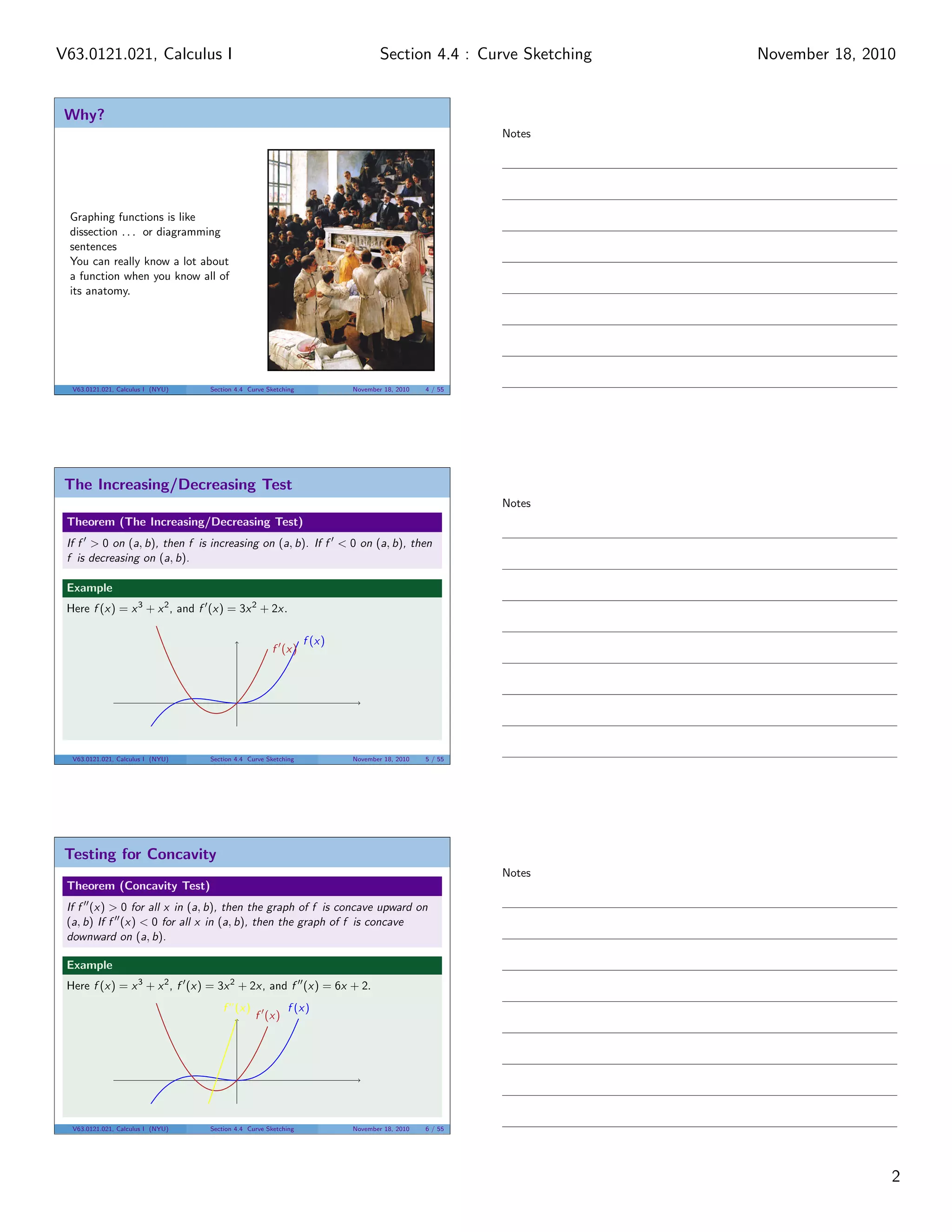
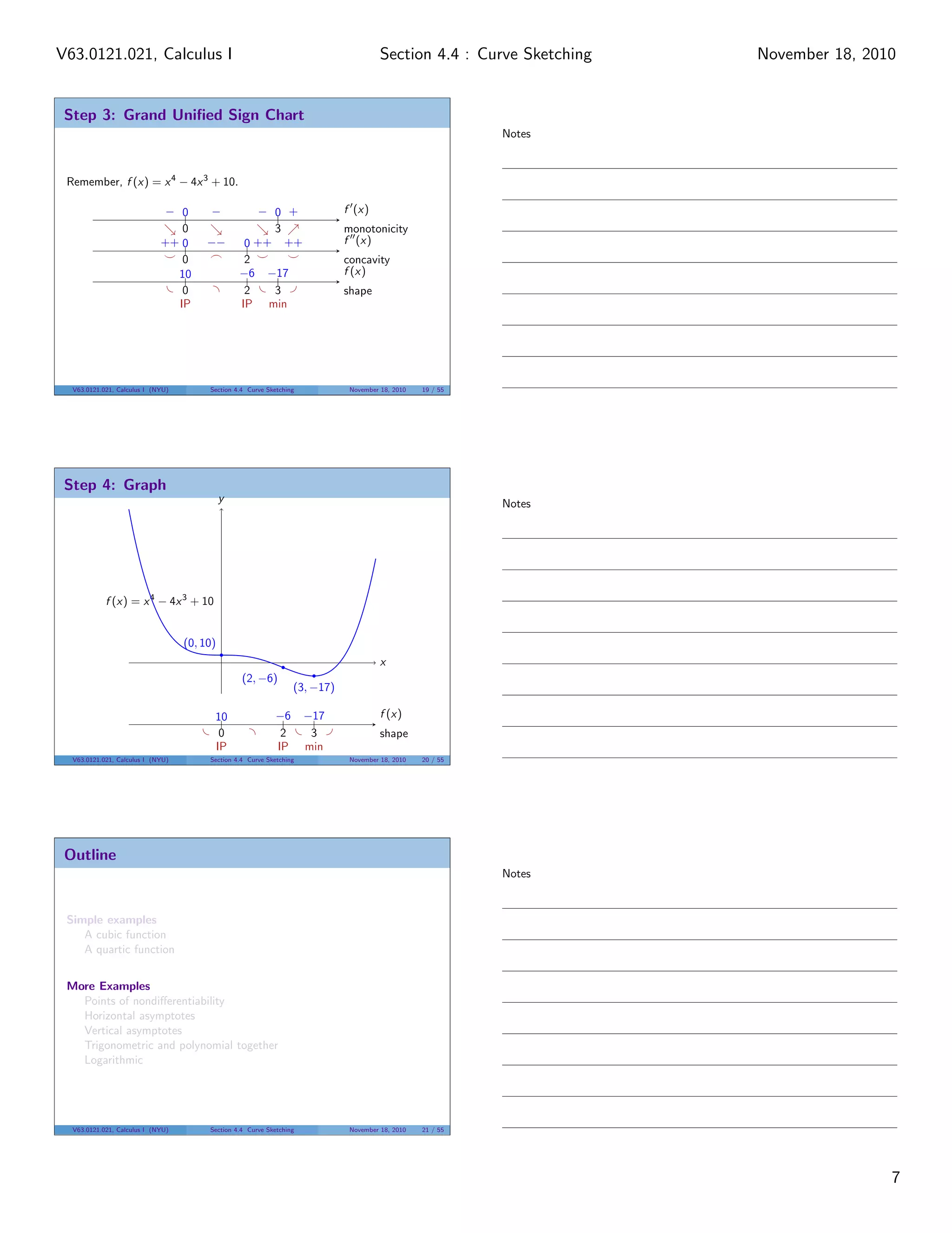
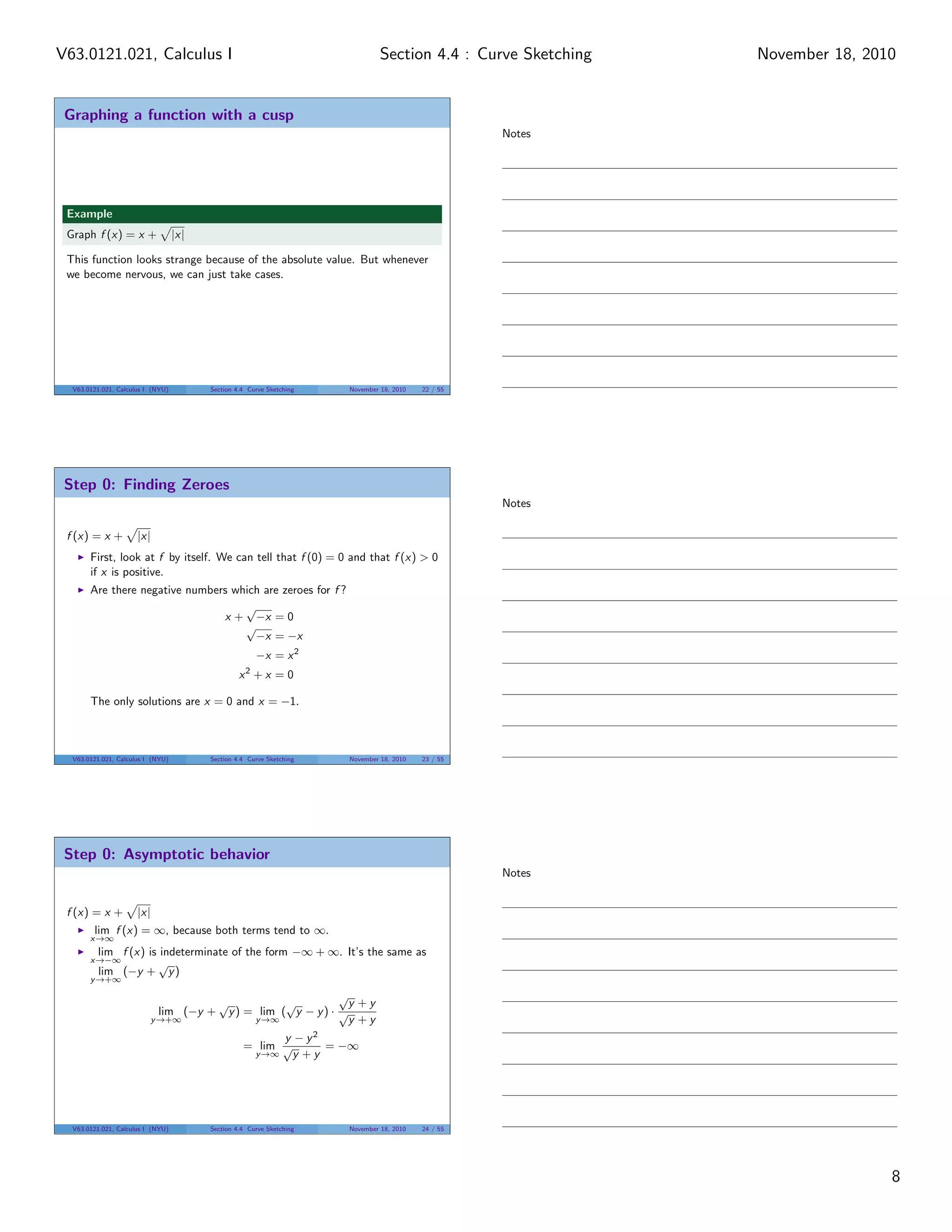
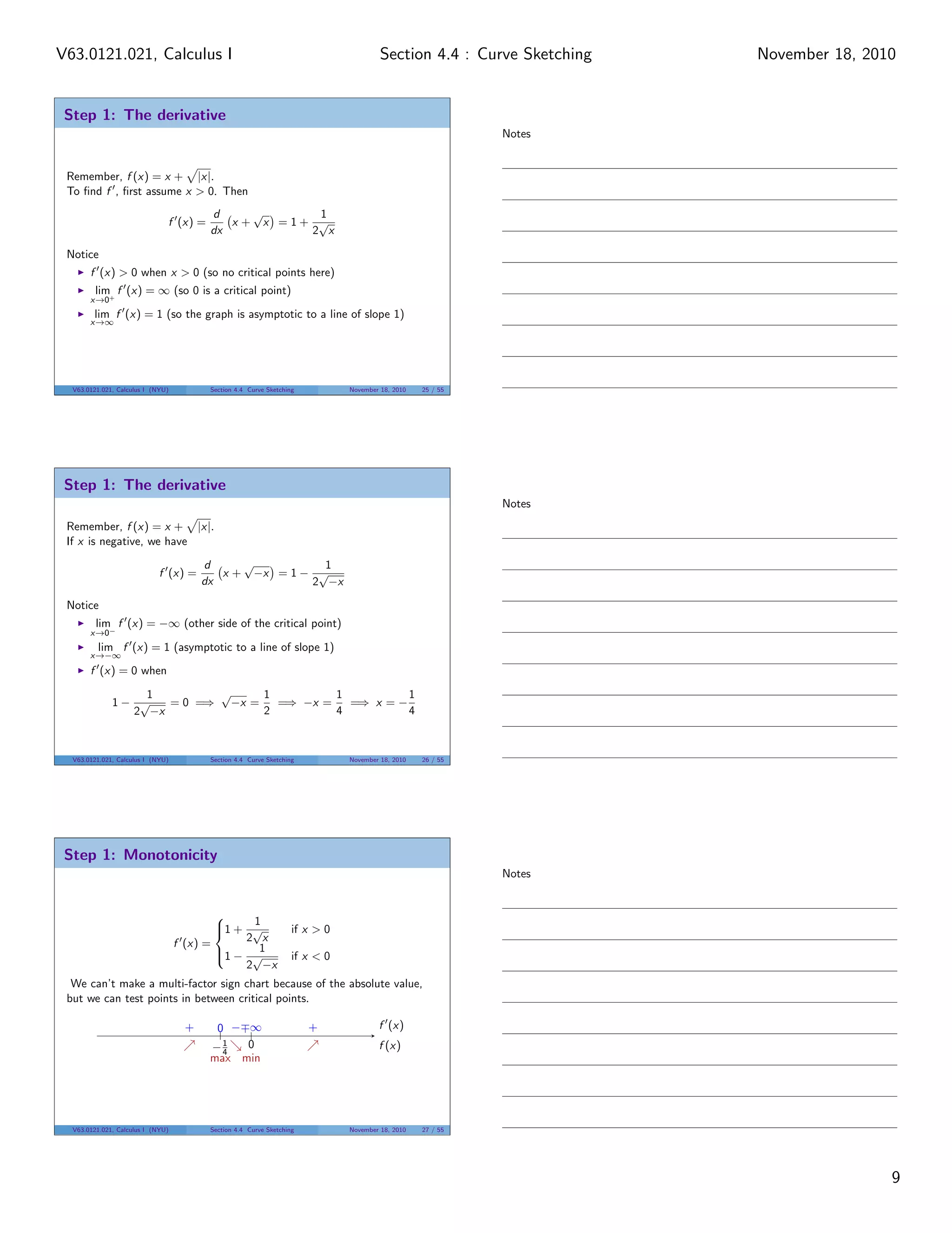
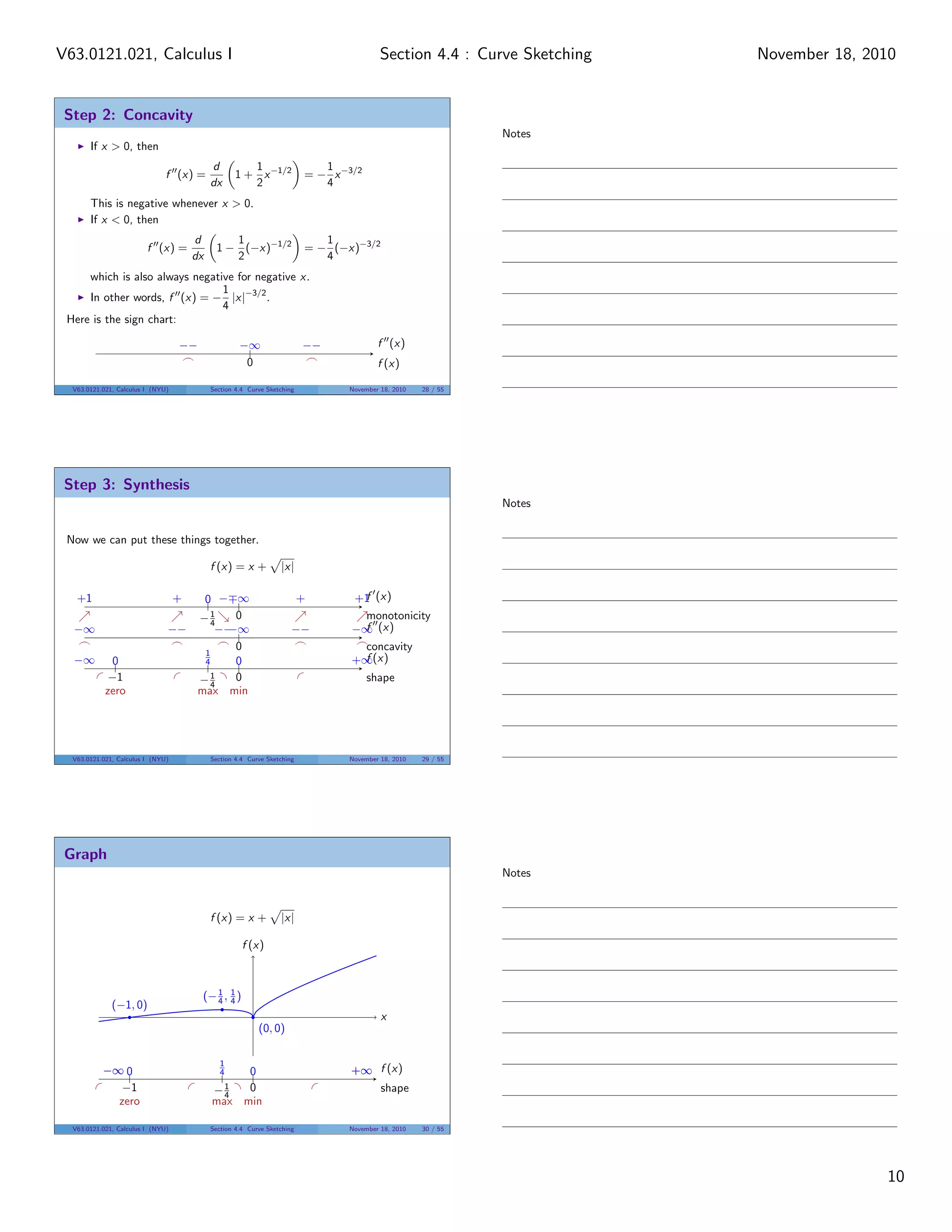


The document provides a detailed lecture on curve sketching for a Calculus I course at New York University. It outlines objectives such as identifying key points on a graph, monotonicity, and concavity, along with practical steps to graph functions, including examples with different types of equations. The notes include tests for increasing/decreasing behavior and concavity, with examples illustrating the application of these concepts.