Download as PDF, PPTX


![The definite integral as a limit
Definition
If f is a function defined on [a, b], the definite integral of f from a to b
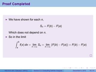
is the number ∫ b ∑n
f(x) dx = lim f(ci ) ∆x
a n→∞
i=1
b−a
where ∆x = , and for each i, xi = a + i∆x, and ci is a point in
n
[xi−1 , xi ].
Theorem
If f is continuous on [a, b] or if f has only finitely many jump
discontinuities, then f is integrable on [a, b]; that is, the definite integral
∫ b
f(x) dx exists and is the same for any choice of ci .
a
. . . . . .
V63.0121.041, Calculus I (NYU) Section 5.3 Evaluating Definite Integrals December 6, 2010 5 / 41](https://image.slidesharecdn.com/lesson25-evaluatingdefiniteintegrals041slides-101206231615-phpapp01/85/Lesson-25-Evaluating-Definite-Integrals-Section-041-slides-5-320.jpg)
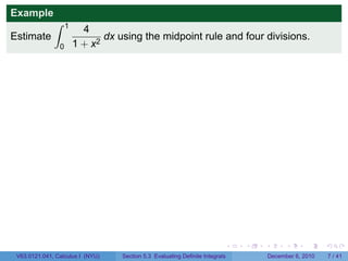
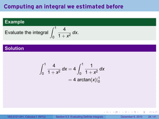
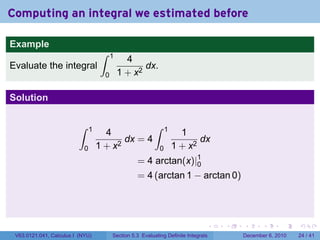
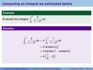
![Example
∫ 1
4
Estimate dx using the midpoint rule and four divisions.
0 1 + x2
Solution
Dividing up [0, 1] into 4 pieces gives
1 2 3 4
x0 = 0, x1 = , x2 = , x3 = , x4 =
4 4 4 4
So the midpoint rule gives
( )
1 4 4 4 4
M4 = + + +
4 1 + (1/8)2 1 + (3/8)2 1 + (5/8)2 1 + (7/8)2
. . . . . .
V63.0121.041, Calculus I (NYU) Section 5.3 Evaluating Definite Integrals December 6, 2010 7 / 41](https://image.slidesharecdn.com/lesson25-evaluatingdefiniteintegrals041slides-101206231615-phpapp01/85/Lesson-25-Evaluating-Definite-Integrals-Section-041-slides-8-320.jpg)
![Example
∫ 1
4
Estimate dx using the midpoint rule and four divisions.
0 1 + x2
Solution
Dividing up [0, 1] into 4 pieces gives
1 2 3 4
x0 = 0, x1 = , x2 = , x3 = , x4 =
4 4 4 4
So the midpoint rule gives
( )
1 4 4 4 4
M4 = + + +
4 1 + (1/8)2 1 + (3/8)2 1 + (5/8)2 1 + (7/8)2
( )
1 4 4 4 4
= + + +
4 65/64 73/64 89/64 113/64
. . . . . .
V63.0121.041, Calculus I (NYU) Section 5.3 Evaluating Definite Integrals December 6, 2010 7 / 41](https://image.slidesharecdn.com/lesson25-evaluatingdefiniteintegrals041slides-101206231615-phpapp01/85/Lesson-25-Evaluating-Definite-Integrals-Section-041-slides-9-320.jpg)
![Example
∫ 1
4
Estimate dx using the midpoint rule and four divisions.
0 1 + x2
Solution
Dividing up [0, 1] into 4 pieces gives
1 2 3 4
x0 = 0, x1 = , x2 = , x3 = , x4 =
4 4 4 4
So the midpoint rule gives
( )
1 4 4 4 4
M4 = + + +
4 1 + (1/8)2 1 + (3/8)2 1 + (5/8)2 1 + (7/8)2
( )
1 4 4 4 4
= + + +
4 65/64 73/64 89/64 113/64
150, 166, 784
= ≈ 3.1468
47, 720, 465
. . . . . .
V63.0121.041, Calculus I (NYU) Section 5.3 Evaluating Definite Integrals December 6, 2010 7 / 41](https://image.slidesharecdn.com/lesson25-evaluatingdefiniteintegrals041slides-101206231615-phpapp01/85/Lesson-25-Evaluating-Definite-Integrals-Section-041-slides-10-320.jpg)
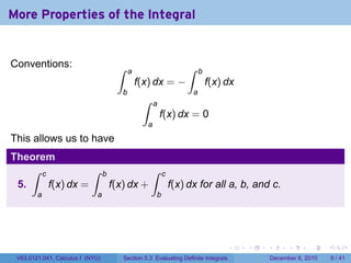
![Properties of the integral
Theorem (Additive Properties of the Integral)
Let f and g be integrable functions on [a, b] and c a constant. Then
∫ b
1. c dx = c(b − a)
a
∫ b ∫ b ∫ b
2. [f(x) + g(x)] dx = f(x) dx + g(x) dx.
a a a
∫ b ∫ b
3. cf(x) dx = c f(x) dx.
a a
∫ b ∫ b ∫ b
4. [f(x) − g(x)] dx = f(x) dx − g(x) dx.
a a a
. . . . . .
V63.0121.041, Calculus I (NYU) Section 5.3 Evaluating Definite Integrals December 6, 2010 8 / 41](https://image.slidesharecdn.com/lesson25-evaluatingdefiniteintegrals041slides-101206231615-phpapp01/85/Lesson-25-Evaluating-Definite-Integrals-Section-041-slides-11-320.jpg)
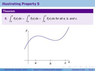


![Comparison Properties of the Integral
Theorem
Let f and g be integrable functions on [a, b].
∫ b
6. If f(x) ≥ 0 for all x in [a, b], then f(x) dx ≥ 0
a
. . . . . .
V63.0121.041, Calculus I (NYU) Section 5.3 Evaluating Definite Integrals December 6, 2010 12 / 41](https://image.slidesharecdn.com/lesson25-evaluatingdefiniteintegrals041slides-101206231615-phpapp01/85/Lesson-25-Evaluating-Definite-Integrals-Section-041-slides-22-320.jpg)
![Comparison Properties of the Integral
Theorem
Let f and g be integrable functions on [a, b].
∫ b
6. If f(x) ≥ 0 for all x in [a, b], then f(x) dx ≥ 0
a
7. If f(x) ≥ g(x) for all x in [a, b], then
∫ b ∫ b
f(x) dx ≥ g(x) dx
a a
. . . . . .
V63.0121.041, Calculus I (NYU) Section 5.3 Evaluating Definite Integrals December 6, 2010 12 / 41](https://image.slidesharecdn.com/lesson25-evaluatingdefiniteintegrals041slides-101206231615-phpapp01/85/Lesson-25-Evaluating-Definite-Integrals-Section-041-slides-23-320.jpg)
![Comparison Properties of the Integral
Theorem
Let f and g be integrable functions on [a, b].
∫ b
6. If f(x) ≥ 0 for all x in [a, b], then f(x) dx ≥ 0
a
7. If f(x) ≥ g(x) for all x in [a, b], then
∫ b ∫ b
f(x) dx ≥ g(x) dx
a a
8. If m ≤ f(x) ≤ M for all x in [a, b], then
∫ b
m(b − a) ≤ f(x) dx ≤ M(b − a)
a
. . . . . .
V63.0121.041, Calculus I (NYU) Section 5.3 Evaluating Definite Integrals December 6, 2010 12 / 41](https://image.slidesharecdn.com/lesson25-evaluatingdefiniteintegrals041slides-101206231615-phpapp01/85/Lesson-25-Evaluating-Definite-Integrals-Section-041-slides-24-320.jpg)
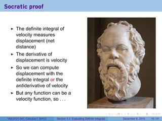
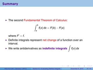
![Theorem of the Day
Theorem (The Second Fundamental Theorem of Calculus)
Suppose f is integrable on [a, b] and f = F′ for another function F, then
∫ b
f(x) dx = F(b) − F(a).
a
. . . . . .
V63.0121.041, Calculus I (NYU) Section 5.3 Evaluating Definite Integrals December 6, 2010 16 / 41](https://image.slidesharecdn.com/lesson25-evaluatingdefiniteintegrals041slides-101206231615-phpapp01/85/Lesson-25-Evaluating-Definite-Integrals-Section-041-slides-29-320.jpg)
![Theorem of the Day
Theorem (The Second Fundamental Theorem of Calculus)
Suppose f is integrable on [a, b] and f = F′ for another function F, then
∫ b
f(x) dx = F(b) − F(a).
a
Note
In Section 5.3, this theorem is called “The Evaluation Theorem”.
Nobody else in the world calls it that.
. . . . . .
V63.0121.041, Calculus I (NYU) Section 5.3 Evaluating Definite Integrals December 6, 2010 16 / 41](https://image.slidesharecdn.com/lesson25-evaluatingdefiniteintegrals041slides-101206231615-phpapp01/85/Lesson-25-Evaluating-Definite-Integrals-Section-041-slides-30-320.jpg)
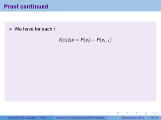
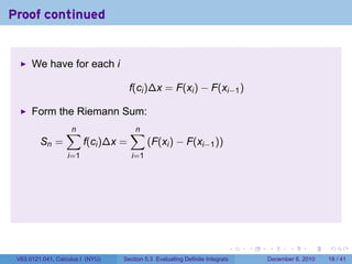
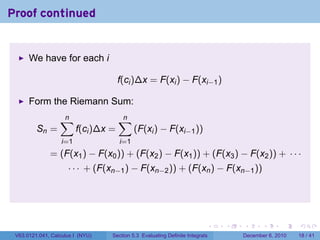
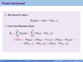
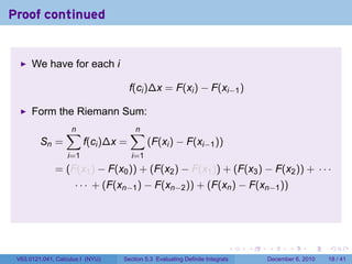
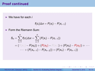
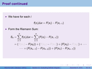
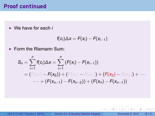
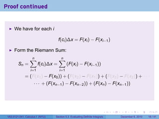
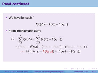
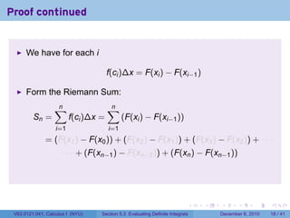
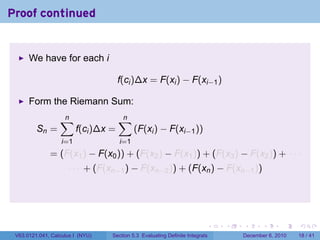
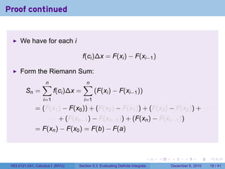
![Proving the Second FTC
b−a
Divide up [a, b] into n pieces of equal width ∆x = as usual.
n
. . . . . .
V63.0121.041, Calculus I (NYU) Section 5.3 Evaluating Definite Integrals December 6, 2010 17 / 41](https://image.slidesharecdn.com/lesson25-evaluatingdefiniteintegrals041slides-101206231615-phpapp01/85/Lesson-25-Evaluating-Definite-Integrals-Section-041-slides-31-320.jpg)
![Proving the Second FTC
b−a
Divide up [a, b] into n pieces of equal width ∆x = as usual.
n
For each i, F is continuous on [xi−1 , xi ] and differentiable on
(xi−1 , xi ). So there is a point ci in (xi−1 , xi ) with
F(xi ) − F(xi−1 )
= F′ (ci ) = f(ci )
xi − xi−1
. . . . . .
V63.0121.041, Calculus I (NYU) Section 5.3 Evaluating Definite Integrals December 6, 2010 17 / 41](https://image.slidesharecdn.com/lesson25-evaluatingdefiniteintegrals041slides-101206231615-phpapp01/85/Lesson-25-Evaluating-Definite-Integrals-Section-041-slides-32-320.jpg)
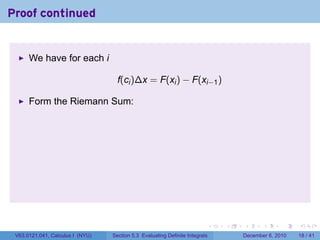
![Proving the Second FTC
b−a
Divide up [a, b] into n pieces of equal width ∆x = as usual.
n
For each i, F is continuous on [xi−1 , xi ] and differentiable on
(xi−1 , xi ). So there is a point ci in (xi−1 , xi ) with
F(xi ) − F(xi−1 )
= F′ (ci ) = f(ci )
xi − xi−1
Or
f(ci )∆x = F(xi ) − F(xi−1 )
. . . . . .
V63.0121.041, Calculus I (NYU) Section 5.3 Evaluating Definite Integrals December 6, 2010 17 / 41](https://image.slidesharecdn.com/lesson25-evaluatingdefiniteintegrals041slides-101206231615-phpapp01/85/Lesson-25-Evaluating-Definite-Integrals-Section-041-slides-33-320.jpg)

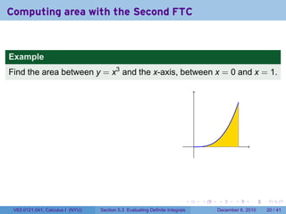
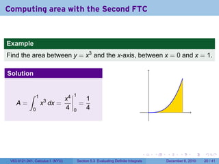
![Computing area with the Second FTC
Example
Find the area between y = x3 and the x-axis, between x = 0 and x = 1.
Solution
∫ 1 1
x4 1
A= x3 dx = =
0 4 0 4 .
Here we use the notation F(x)|b or [F(x)]b to mean F(b) − F(a).
a a
. . . . . .
V63.0121.041, Calculus I (NYU) Section 5.3 Evaluating Definite Integrals December 6, 2010 20 / 41](https://image.slidesharecdn.com/lesson25-evaluatingdefiniteintegrals041slides-101206231615-phpapp01/85/Lesson-25-Evaluating-Definite-Integrals-Section-041-slides-53-320.jpg)
![Computing area with the Second FTC
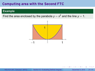
Example
Find the area enclosed by the parabola y = x2 and the line y = 1.
1
.
−1 1
Solution
∫ 1 [ ]1 ( [ )]
x3 1 1 4
A=2− x dx = 2 − 2
=2− − − =
−1 3 −1 3 3 3
. . . . . .
V63.0121.041, Calculus I (NYU) Section 5.3 Evaluating Definite Integrals December 6, 2010 21 / 41](https://image.slidesharecdn.com/lesson25-evaluatingdefiniteintegrals041slides-101206231615-phpapp01/85/Lesson-25-Evaluating-Definite-Integrals-Section-041-slides-56-320.jpg)
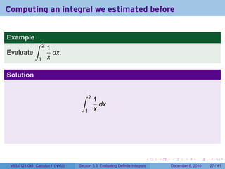
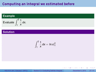
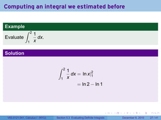
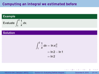
![Example
∫ 1
4
Estimate dx using the midpoint rule and four divisions.
0 1 + x2
Solution
Dividing up [0, 1] into 4 pieces gives
1 2 3 4
x0 = 0, x1 = , x2 = , x3 = , x4 =
4 4 4 4
So the midpoint rule gives
( )
1 4 4 4 4
M4 = + + +
4 1 + (1/8)2 1 + (3/8)2 1 + (5/8)2 1 + (7/8)2
( )
1 4 4 4 4
= + + +
4 65/64 73/64 89/64 113/64
150, 166, 784
= ≈ 3.1468
47, 720, 465
. . . . . .
V63.0121.041, Calculus I (NYU) Section 5.3 Evaluating Definite Integrals December 6, 2010 23 / 41](https://image.slidesharecdn.com/lesson25-evaluatingdefiniteintegrals041slides-101206231615-phpapp01/85/Lesson-25-Evaluating-Definite-Integrals-Section-041-slides-58-320.jpg)


![My first table of integrals
.
∫ ∫ ∫
[f(x) + g(x)] dx = f(x) dx + g(x) dx
∫ ∫ ∫
xn+1
n
x dx = + C (n ̸= −1) cf(x) dx = c f(x) dx
n+1 ∫
∫
1
ex dx = ex + C dx = ln |x| + C
x
∫ ∫
ax
sin x dx = − cos x + C ax dx = +C
ln a
∫ ∫
cos x dx = sin x + C csc2 x dx = − cot x + C
∫ ∫
sec2 x dx = tan x + C csc x cot x dx = − csc x + C
∫ ∫
1
sec x tan x dx = sec x + C √ dx = arcsin x + C
∫ 1 − x2
1
dx = arctan x + C
1 + x2
. . . . . .
V63.0121.041, Calculus I (NYU) Section 5.3 Evaluating Definite Integrals December 6, 2010 32 / 41](https://image.slidesharecdn.com/lesson25-evaluatingdefiniteintegrals041slides-101206231615-phpapp01/85/Lesson-25-Evaluating-Definite-Integrals-Section-041-slides-78-320.jpg)
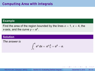
![Computing Area with integrals
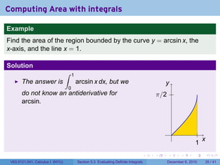
Example
Find the area of the region bounded by the curve y = arcsin x, the
x-axis, and the line x = 1.
Solution
∫ 1
The answer is arcsin x dx, but we y
0
do not know an antiderivative for π/2
arcsin.
Instead compute the area as
∫ π/2
π π π/2
− sin y dy = −[− cos x]0 .
2 0 2
x
1
. . . . . .
V63.0121.041, Calculus I (NYU) Section 5.3 Evaluating Definite Integrals December 6, 2010 35 / 41](https://image.slidesharecdn.com/lesson25-evaluatingdefiniteintegrals041slides-101206231615-phpapp01/85/Lesson-25-Evaluating-Definite-Integrals-Section-041-slides-85-320.jpg)
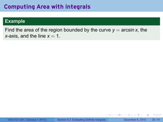
![Computing Area with integrals
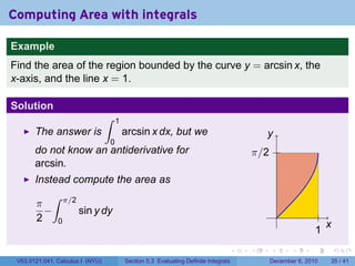
Example
Find the area of the region bounded by the curve y = arcsin x, the
x-axis, and the line x = 1.
Solution
∫ 1
The answer is arcsin x dx, but we y
0
do not know an antiderivative for π/2
arcsin.
Instead compute the area as
∫ π/2
π π π/2 π
− sin y dy = −[− cos x]0 = −1 .
2 0 2 2
x
1
. . . . . .
V63.0121.041, Calculus I (NYU) Section 5.3 Evaluating Definite Integrals December 6, 2010 35 / 41](https://image.slidesharecdn.com/lesson25-evaluatingdefiniteintegrals041slides-101206231615-phpapp01/85/Lesson-25-Evaluating-Definite-Integrals-Section-041-slides-86-320.jpg)
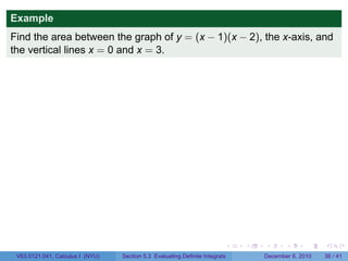
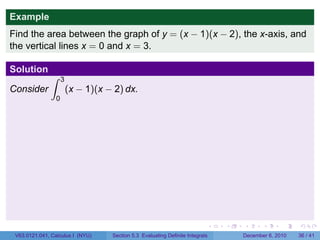
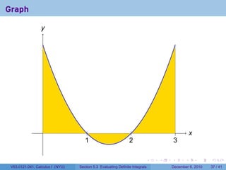
![Example
Find the area between the graph of y = (x − 1)(x − 2), the x-axis, and
the vertical lines x = 0 and x = 3.
Solution
∫ 3
Consider (x − 1)(x − 2) dx. Notice the integrand is positive on [0, 1)
0
and (2, 3], and negative on (1, 2).
. . . . . .
V63.0121.041, Calculus I (NYU) Section 5.3 Evaluating Definite Integrals December 6, 2010 38 / 41](https://image.slidesharecdn.com/lesson25-evaluatingdefiniteintegrals041slides-101206231615-phpapp01/85/Lesson-25-Evaluating-Definite-Integrals-Section-041-slides-90-320.jpg)
![Example
Find the area between the graph of y = (x − 1)(x − 2), the x-axis, and
the vertical lines x = 0 and x = 3.
Solution
∫ 3
Consider (x − 1)(x − 2) dx. Notice the integrand is positive on [0, 1)
0
and (2, 3], and negative on (1, 2). If we want the area of the region, we
have to do
∫ 1 ∫ 2 ∫ 3
A= (x − 1)(x − 2) dx − (x − 1)(x − 2) dx + (x − 1)(x − 2) dx
0 1 2
[ ]1 [ ]2 [ ]3
= − 1 3
3x
3 2
2x + 2x − 1 x3 − 3 x2 + 2x + 1 x3 − 3 x2 + 2x
3 2 3 2
( ) 0 1 2
5 1 5 11
= − − + = .
6 6 6 6
. . . . . .
V63.0121.041, Calculus I (NYU) Section 5.3 Evaluating Definite Integrals December 6, 2010 38 / 41](https://image.slidesharecdn.com/lesson25-evaluatingdefiniteintegrals041slides-101206231615-phpapp01/85/Lesson-25-Evaluating-Definite-Integrals-Section-041-slides-91-320.jpg)
![What about the constant?
It seems we forgot about the +C when we say for instance
∫ 1 1
x4 1 1
3
x dx = = −0=
0 4 0 4 4
But notice
[ 4 ]1 ( )
x 1 1 1
+C = + C − (0 + C) = + C − C =
4 0 4 4 4
no matter what C is.
So in antidifferentiation for definite integrals, the constant is
immaterial.
. . . . . .
V63.0121.041, Calculus I (NYU) Section 5.3 Evaluating Definite Integrals December 6, 2010 40 / 41](https://image.slidesharecdn.com/lesson25-evaluatingdefiniteintegrals041slides-101206231615-phpapp01/85/Lesson-25-Evaluating-Definite-Integrals-Section-041-slides-93-320.jpg)

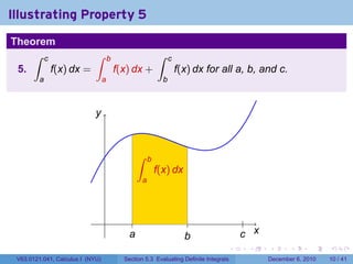
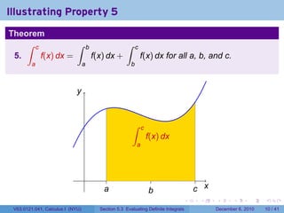
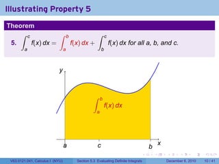
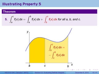
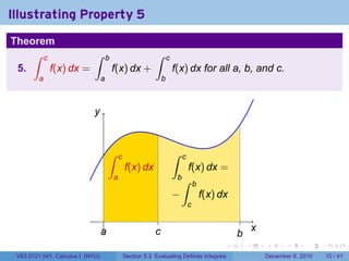
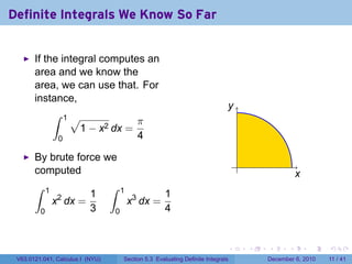
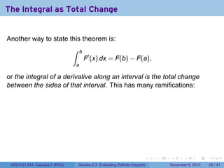
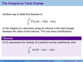
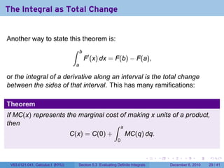
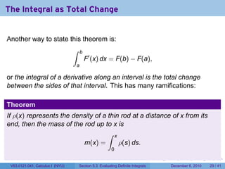
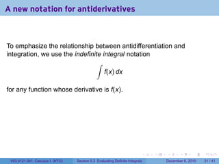
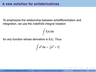
This document outlines a calculus lecture on evaluating definite integrals. The lecture will: 1) Use the Evaluation Theorem to evaluate definite integrals and write antiderivatives as indefinite integrals. 2) Interpret definite integrals as the "net change" of a function over an interval. 3) Provide examples of evaluating definite integrals and estimating integrals using the midpoint rule. 4) Discuss properties of integrals such as additivity and illustrate how a definite integral from a to c can be broken into integrals from a to b and b to c.