Downloaded 26 times
![Objectives
Use the second derivative of
a function to determine the
intervals along which the
graph of the function is
concave up or concave down
(The Concavity Test)
Use the first and second
derivative of a function to
classify critical points as
local maxima or local
minima, when applicable
(The Second Derivative
Test)
V63.0121.041, Calculus I (NYU) Section 4.2 The Shapes of Curves November 15, 2010 4 / 31
Outline
Recall: The Mean Value Theorem
Monotonicity
The Increasing/Decreasing Test
Finding intervals of monotonicity
The First Derivative Test
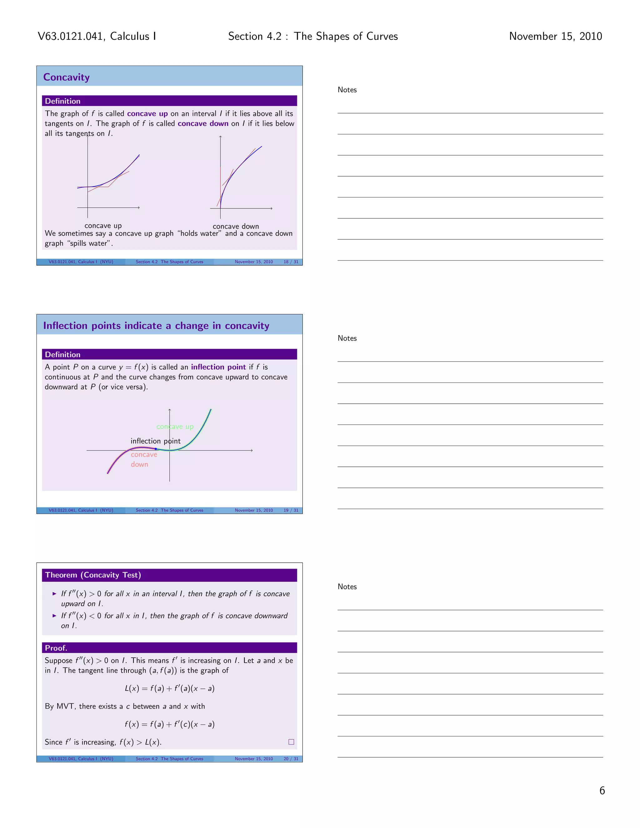
Concavity
Definitions
Testing for Concavity
The Second Derivative Test
V63.0121.041, Calculus I (NYU) Section 4.2 The Shapes of Curves November 15, 2010 5 / 31
Recall: The Mean Value Theorem
Theorem (The Mean Value Theorem)
Let f be continuous on [a, b] and
differentiable on (a, b). Then
there exists a point c in (a, b)
such that
f (b) − f (a)
b − a
= f (c).
a
b
c
Another way to put this is that there exists a point c such that
f (b) = f (a) + f (c)(b − a)
V63.0121.041, Calculus I (NYU) Section 4.2 The Shapes of Curves November 15, 2010 6 / 31
Notes
Notes
Notes
2
Section 4.2 : The Shapes of CurvesV63.0121.041, Calculus I November 15, 2010](https://image.slidesharecdn.com/lesson20-derivativesandtheshapeofcurves041handout-101114213320-phpapp01/75/Lesson-20-Derivatives-and-the-Shape-of-Curves-Section-041-handout-2-2048.jpg)
![Why the MVT is the MITC
Most Important Theorem In Calculus!
Theorem
Let f = 0 on an interval (a, b). Then f is constant on (a, b).
Proof.
Pick any points x and y in (a, b) with x < y. Then f is continuous on
[x, y] and differentiable on (x, y). By MVT there exists a point z in (x, y)
such that
f (y) = f (x) + f (z)(y − x)
So f (y) = f (x). Since this is true for all x and y in (a, b), then f is
constant.
V63.0121.041, Calculus I (NYU) Section 4.2 The Shapes of Curves November 15, 2010 7 / 31
Outline
Recall: The Mean Value Theorem
Monotonicity
The Increasing/Decreasing Test
Finding intervals of monotonicity
The First Derivative Test
Concavity
Definitions
Testing for Concavity
The Second Derivative Test
V63.0121.041, Calculus I (NYU) Section 4.2 The Shapes of Curves November 15, 2010 8 / 31
What does it mean for a function to be increasing?
Definition
A function f is increasing on (a, b) if
f (x) < f (y)
whenever x and y are two points in (a, b) with x < y.
An increasing function “preserves order.”
Write your own definition (mutatis mutandis) of decreasing,
nonincreasing, nondecreasing
V63.0121.041, Calculus I (NYU) Section 4.2 The Shapes of Curves November 15, 2010 9 / 31
Notes
Notes
Notes
3
Section 4.2 : The Shapes of CurvesV63.0121.041, Calculus I November 15, 2010](https://image.slidesharecdn.com/lesson20-derivativesandtheshapeofcurves041handout-101114213320-phpapp01/75/Lesson-20-Derivatives-and-the-Shape-of-Curves-Section-041-handout-3-2048.jpg)
![The Increasing/Decreasing Test
Theorem (The Increasing/Decreasing Test)
If f > 0 on (a, b), then f is increasing on (a, b). If f < 0 on (a, b), then
f is decreasing on (a, b).
Proof.
It works the same as the last theorem. Pick two points x and y in (a, b)
with x < y. We must show f (x) < f (y). By MVT there exists a point c
in (x, y) such that
f (y) − f (x) = f (c)(y − x) > 0.
So f (y) > f (x).
V63.0121.041, Calculus I (NYU) Section 4.2 The Shapes of Curves November 15, 2010 10 / 31
Finding intervals of monotonicity I
Example
Find the intervals of monotonicity of f (x) = 2x − 5.
Solution
f (x) = 2 is always positive, so f is increasing on (−∞, ∞).
Example
Describe the monotonicity of f (x) = arctan(x).
Solution
Since f (x) =
1
1 + x2
is always positive, f (x) is always increasing.
V63.0121.041, Calculus I (NYU) Section 4.2 The Shapes of Curves November 15, 2010 11 / 31
Finding intervals of monotonicity II
Example
Find the intervals of monotonicity of f (x) = x2
− 1.
Solution
f (x) = 2x, which is positive when x > 0 and negative when x is.
We can draw a number line:
f
f
−
0
0 +
So f is decreasing on (−∞, 0) and increasing on (0, ∞).
In fact we can say f is decreasing on (−∞, 0] and increasing on [0, ∞)
V63.0121.041, Calculus I (NYU) Section 4.2 The Shapes of Curves November 15, 2010 12 / 31
Notes
Notes
Notes
4
Section 4.2 : The Shapes of CurvesV63.0121.041, Calculus I November 15, 2010](https://image.slidesharecdn.com/lesson20-derivativesandtheshapeofcurves041handout-101114213320-phpapp01/75/Lesson-20-Derivatives-and-the-Shape-of-Curves-Section-041-handout-4-2048.jpg)
![Finding intervals of monotonicity III
Example
Find the intervals of monotonicity of f (x) = x2/3
(x + 2).
Solution
V63.0121.041, Calculus I (NYU) Section 4.2 The Shapes of Curves November 15, 2010 13 / 31
The First Derivative Test
Theorem (The First Derivative Test)
Let f be continuous on [a, b] and c a critical point of f in (a, b).
If f (x) > 0 on (a, c) and f (x) < 0 on (c, b), then c is a local
maximum.
If f (x) < 0 on (a, c) and f (x) > 0 on (c, b), then c is a local
minimum.
If f (x) has the same sign on (a, c) and (c, b), then c is not a local
extremum.
V63.0121.041, Calculus I (NYU) Section 4.2 The Shapes of Curves November 15, 2010 14 / 31
Outline
Recall: The Mean Value Theorem
Monotonicity
The Increasing/Decreasing Test
Finding intervals of monotonicity
The First Derivative Test
Concavity
Definitions
Testing for Concavity
The Second Derivative Test
V63.0121.041, Calculus I (NYU) Section 4.2 The Shapes of Curves November 15, 2010 17 / 31
Notes
Notes
Notes
5
Section 4.2 : The Shapes of CurvesV63.0121.041, Calculus I November 15, 2010](https://image.slidesharecdn.com/lesson20-derivativesandtheshapeofcurves041handout-101114213320-phpapp01/75/Lesson-20-Derivatives-and-the-Shape-of-Curves-Section-041-handout-5-2048.jpg)
![Finding Intervals of Concavity I
Example
Find the intervals of concavity for the graph of f (x) = x3
+ x2
.
Solution
We have f (x) = 3x2
+ 2x, so f (x) = 6x + 2.
This is negative when x < −1/3, positive when x > −1/3, and 0 when
x = −1/3
So f is concave down on (−∞, −1/3), concave up on (−1/3, ∞), and
has an inflection point at (−1/3, 2/27)
V63.0121.041, Calculus I (NYU) Section 4.2 The Shapes of Curves November 15, 2010 21 / 31
Finding Intervals of Concavity II
Example
Find the intervals of concavity of the graph of f (x) = x2/3
(x + 2).
Solution
V63.0121.041, Calculus I (NYU) Section 4.2 The Shapes of Curves November 15, 2010 22 / 31
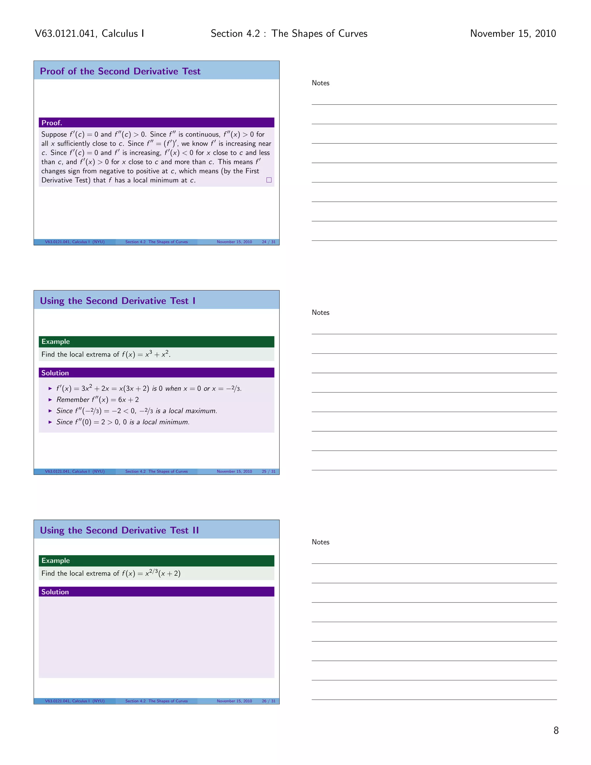
The Second Derivative Test
Theorem (The Second Derivative Test)
Let f , f , and f be continuous on [a, b]. Let c be be a point in (a, b)
with f (c) = 0.
If f (c) < 0, then c is a local maximum.
If f (c) > 0, then c is a local minimum.
Remarks
If f (c) = 0, the second derivative test is inconclusive (this does not
mean c is neither; we just don’t know yet).
We look for zeroes of f and plug them into f to determine if their f
values are local extreme values.
V63.0121.041, Calculus I (NYU) Section 4.2 The Shapes of Curves November 15, 2010 23 / 31
Notes
Notes
Notes
7
Section 4.2 : The Shapes of CurvesV63.0121.041, Calculus I November 15, 2010](https://image.slidesharecdn.com/lesson20-derivativesandtheshapeofcurves041handout-101114213320-phpapp01/75/Lesson-20-Derivatives-and-the-Shape-of-Curves-Section-041-handout-7-2048.jpg)

1) The document discusses using derivatives to determine the shapes of curves, including intervals of increasing/decreasing behavior, local extrema, and concavity. 2) Key tests covered are the increasing/decreasing test, first derivative test, concavity test, and second derivative test. These allow determining monotonicity, local extrema, and concavity from the signs of the first and second derivatives. 3) Examples demonstrate applying these tests to find the intervals of monotonicity, points of local extrema, and intervals of concavity for various functions.