The document discusses spatial transformations and intensity transformations for image enhancement. Spatial transformations include scaling, rotation, translation, and shear, which can be represented using a matrix. Intensity transformations modify pixel intensities based on a transfer function and are used for contrast enhancement. Common transformations include image negative, powers, and logarithms. The appropriate transformation depends on the image content and which intensity values need enhancement.


![Image enhancement
Image enhancement is a pre-processing step that makes the
input image better suited for further processing. For example,
for segmentation, recognition, or simply better for somebody
to view the image.
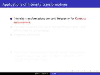
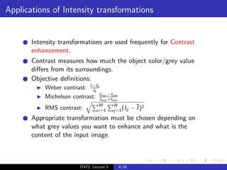
Intensity transformations: Depends only on the intensity value
at a point: g (x, y ) = T [f (x, y )], can be also written as
s = T [r ], where r and s are the input and output grey values
respectively.
IT472: Lecture 5 6/18](https://image.slidesharecdn.com/lecture4-120203150819-phpapp01/85/Image-Processing-3-16-320.jpg)
![Image enhancement
Image enhancement is a pre-processing step that makes the
input image better suited for further processing. For example,
for segmentation, recognition, or simply better for somebody
to view the image.
Intensity transformations: Depends only on the intensity value
at a point: g (x, y ) = T [f (x, y )], can be also written as
s = T [r ], where r and s are the input and output grey values
respectively.
IT472: Lecture 5 6/18](https://image.slidesharecdn.com/lecture4-120203150819-phpapp01/85/Image-Processing-3-17-320.jpg)