Downloaded 45 times


![Why the MVT is the MITC
Most Important Theorem In Calculus!
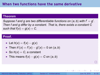
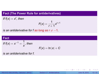
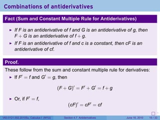
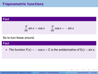
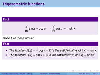
Theorem
Let f′ = 0 on an interval (a, b). Then f is constant on (a, b).
Proof.
Pick any points x and y in (a, b) with x y. Then f is continuous on
[x, y] and differentiable on (x, y). By MVT there exists a point z in (x, y)
such that
f(y) − f(x)
= f′ (z) =⇒ f(y) = f(x) + f′ (z)(y − x)
y−x
But f′ (z) = 0, so f(y) = f(x). Since this is true for all x and y in (a, b),
then f is constant.
. . . . . .
V63.0121.002.2010Su, Calculus I (NYU) Section 4.7 Antiderivatives June 16, 2010 7 / 33](https://image.slidesharecdn.com/lesson23-antiderivativesslides-100615222943-phpapp02/85/Lesson-23-Antiderivatives-13-320.jpg)


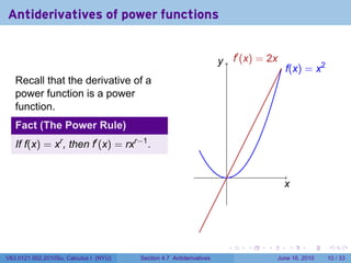
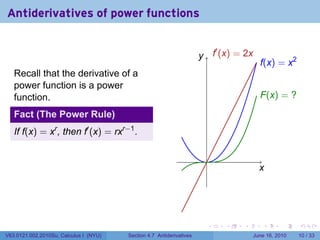


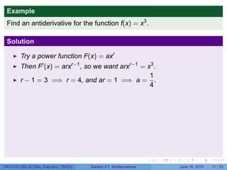
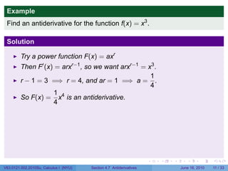
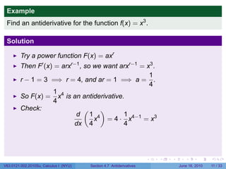
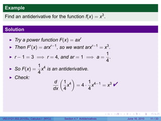
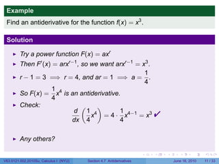
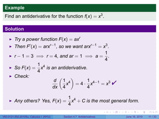


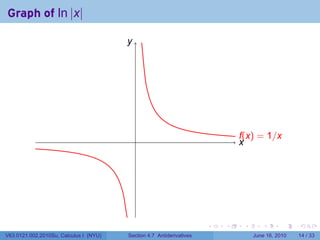
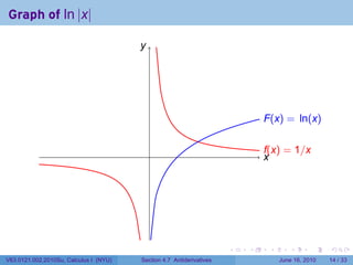
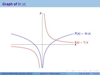
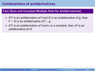


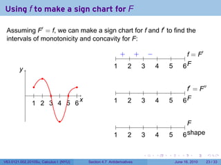
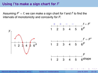
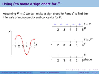
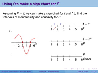


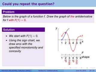

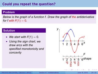


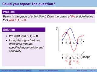

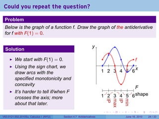


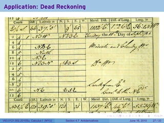
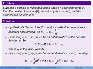


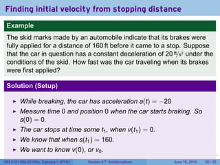
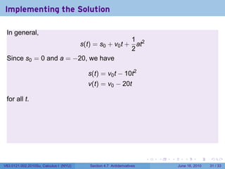
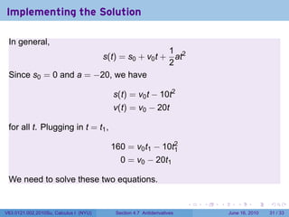

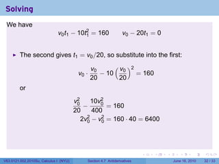

This document is from a Calculus I class at New York University and covers antiderivatives. It begins with announcements about an upcoming quiz. The objectives are to find antiderivatives of simple functions, remember that a function whose derivative is zero must be constant, and solve rectilinear motion problems. It then outlines finding antiderivatives through tabulation, graphically, and with rectilinear motion examples. Examples are provided of finding the antiderivative of power functions like x^3 through identifying the power rule relationship between a function and its derivative.