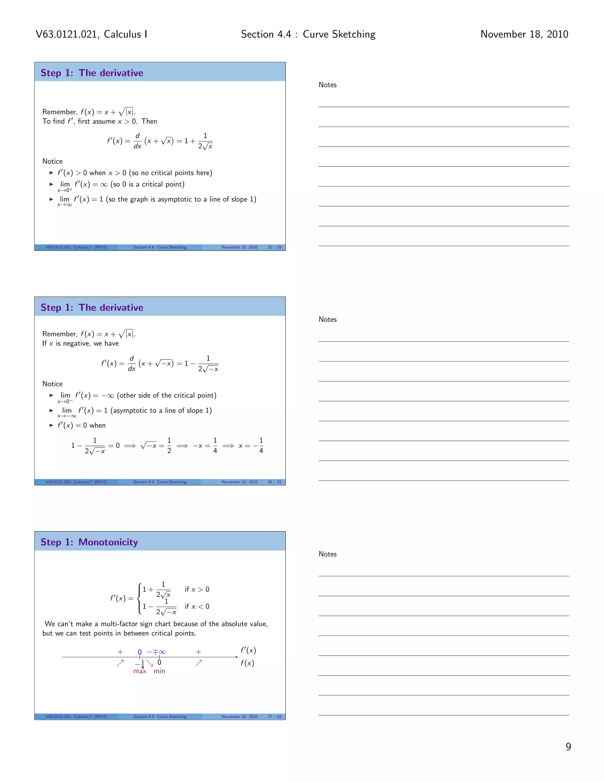
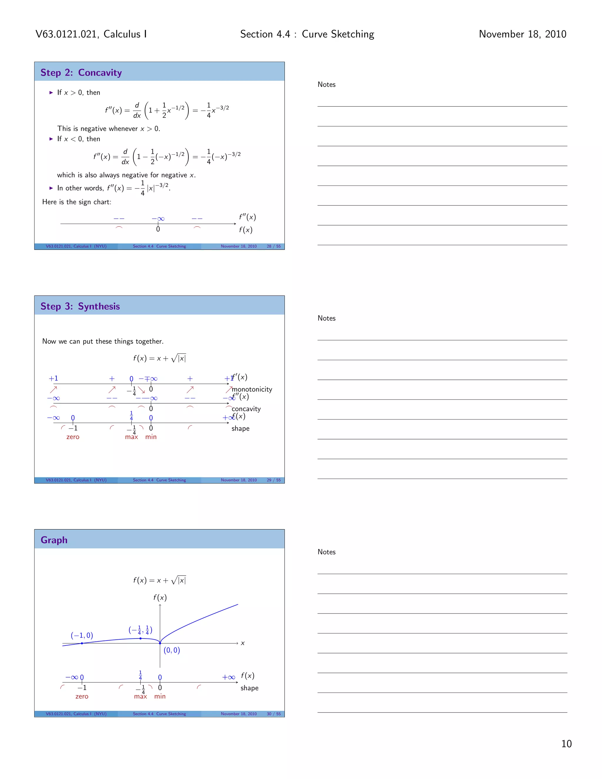
Section 4.4
Curve Sketching
V63.0121.021, Calculus I
New York University
November 18, 2010
Announcements
There is class on November 23. The homework is due on
November 24. Turn in homework to my mailbox or bring to class on
November 23.
Announcements
There is class on
November 23. The
homework is due on
November 24. Turn in
homework to my mailbox or
bring to class on
November 23.
V63.0121.021, Calculus I (NYU) Section 4.4 Curve Sketching November 18, 2010 2 / 55
Objectives
given a function, graph it
completely, indicating
zeroes (if easy)
asymptotes if applicable
critical points
local/global max/min
inflection points
V63.0121.021, Calculus I (NYU) Section 4.4 Curve Sketching November 18, 2010 3 / 55
Notes
Notes
Notes
1
Section 4.4 : Curve SketchingV63.0121.021, Calculus I November 18, 2010
Why?
Graphing functions is like
dissection . . . or diagramming
sentences
You can really know a lot about
a function when you know all of
its anatomy.
V63.0121.021, Calculus I (NYU) Section 4.4 Curve Sketching November 18, 2010 4 / 55
The Increasing/Decreasing Test
Theorem (The Increasing/Decreasing Test)
If f > 0 on (a, b), then f is increasing on (a, b). If f < 0 on (a, b), then
f is decreasing on (a, b).
Example
Here f (x) = x3
+ x2
, and f (x) = 3x2
+ 2x.
f (x)
f (x)
V63.0121.021, Calculus I (NYU) Section 4.4 Curve Sketching November 18, 2010 5 / 55
Testing for Concavity
Theorem (Concavity Test)
If f (x) > 0 for all x in (a, b), then the graph of f is concave upward on
(a, b) If f (x) < 0 for all x in (a, b), then the graph of f is concave
downward on (a, b).
Example
Here f (x) = x3
+ x2
, f (x) = 3x2
+ 2x, and f (x) = 6x + 2.
f (x)
f (x)
f (x)
V63.0121.021, Calculus I (NYU) Section 4.4 Curve Sketching November 18, 2010 6 / 55
Notes
Notes
Notes
2
Section 4.4 : Curve SketchingV63.0121.021, Calculus I November 18, 2010
Graphing Checklist
To graph a function f , follow this plan:
0. Find when f is positive, negative, zero, not
defined.
1. Find f and form its sign chart. Conclude
information about increasing/decreasing
and local max/min.
2. Find f and form its sign chart. Conclude
concave up/concave down and inflection.
3. Put together a big chart to assemble
monotonicity and concavity data
4. Graph!
V63.0121.021, Calculus I (NYU) Section 4.4 Curve Sketching November 18, 2010 7 / 55
Outline
Simple examples
A cubic function
A quartic function
More Examples
Points of nondifferentiability
Horizontal asymptotes
Vertical asymptotes
Trigonometric and polynomial together
Logarithmic
V63.0121.021, Calculus I (NYU) Section 4.4 Curve Sketching November 18, 2010 8 / 55
Graphing a cubic
Example
Graph f (x) = 2x3
− 3x2
− 12x.
(Step 0) First, let’s find the zeros. We can at least factor out one power of
x:
f (x) = x(2x2
− 3x − 12)
so f (0) = 0. The other factor is a quadratic, so we the other two roots are
x =
3 ± 32 − 4(2)(−12)
4
=
3 ±
√
105
4
It’s OK to skip this step for now since the roots are so complicated.
V63.0121.021, Calculus I (NYU) Section 4.4 Curve Sketching November 18, 2010 9 / 55
Notes
Notes
Notes
3
Section 4.4 : Curve SketchingV63.0121.021, Calculus I November 18, 2010
Step 1: Monotonicity
f (x) = 2x3
− 3x2
− 12x
=⇒ f (x) = 6x2
− 6x − 12 = 6(x + 1)(x − 2)
We can form a sign chart from this:
x − 2
2
− − +
x + 1
−1
++−
f (x)
f (x)2−1
+ − +
max min
V63.0121.021, Calculus I (NYU) Section 4.4 Curve Sketching November 18, 2010 10 / 55
Step 2: Concavity
f (x) = 6x2
− 6x − 12
=⇒ f (x) = 12x − 6 = 6(2x − 1)
Another sign chart:
f (x)
f (x)1/2
−− ++
IP
V63.0121.021, Calculus I (NYU) Section 4.4 Curve Sketching November 18, 2010 11 / 55
Step 3: One sign chart to rule them all
Remember, f (x) = 2x3
− 3x2
− 12x.
f (x)
monotonicity−1 2
+− −+
f (x)
concavity1/2
−− −− ++ ++
f (x)
shape of f−1
7
max
2
−20
min
1/2
−61/2
IP
V63.0121.021, Calculus I (NYU) Section 4.4 Curve Sketching November 18, 2010 12 / 55
Notes
Notes
Notes
4
Section 4.4 : Curve SketchingV63.0121.021, Calculus I November 18, 2010
Combinations of monotonicity and concavity
III
III IV
decreasing,
concave
down
increasing,
concave
down
decreasing,
concave up
increasing,
concave up
V63.0121.021, Calculus I (NYU) Section 4.4 Curve Sketching November 18, 2010 13 / 55
Step 3: One sign chart to rule them all
Remember, f (x) = 2x3
− 3x2
− 12x.
f (x)
monotonicity−1 2
+− −+
f (x)
concavity1/2
−− −− ++ ++
f (x)
shape of f−1
7
max
2
−20
min
1/2
−61/2
IP
V63.0121.021, Calculus I (NYU) Section 4.4 Curve Sketching November 18, 2010 14 / 55
Step 4: Graph
f (x) = 2x3
− 3x2
− 12x
x
f (x)
f (x)
shape of f−1
7
max
2
−20
min
1/2
−61/2
IP
3−
√
105
4 , 0
(−1, 7)
(0, 0)
(1/2, −61/2)
(2, −20)
3+
√
105
4 , 0
V63.0121.021, Calculus I (NYU) Section 4.4 Curve Sketching November 18, 2010 15 / 55
Notes
Notes
Notes
5
Section 4.4 : Curve SketchingV63.0121.021, Calculus I November 18, 2010
Graphing a quartic
Example
Graph f (x) = x4
− 4x3
+ 10
(Step 0) We know f (0) = 10 and lim
x→±∞
f (x) = +∞. Not too many other
points on the graph are evident.
V63.0121.021, Calculus I (NYU) Section 4.4 Curve Sketching November 18, 2010 16 / 55
Step 1: Monotonicity
f (x) = x4
− 4x3
+ 10
=⇒ f (x) = 4x3
− 12x2
= 4x2
(x − 3)
We make its sign chart.
4x2
0
0+ + +
(x − 3)
3
0− − +
f (x)
f (x)3
0
0
0− − +
min
V63.0121.021, Calculus I (NYU) Section 4.4 Curve Sketching November 18, 2010 17 / 55
Step 2: Concavity
f (x) = 4x3
− 12x2
=⇒ f (x) = 12x2
− 24x = 12x(x − 2)
Here is its sign chart:
12x
0
0− + +
x − 2
2
0− − +
f (x)
f (x)0
0
2
0++ −− ++
IP IP
V63.0121.021, Calculus I (NYU) Section 4.4 Curve Sketching November 18, 2010 18 / 55
Notes
Notes
Notes
6
Section 4.4 : Curve SketchingV63.0121.021, Calculus I November 18, 2010
Step 3: Grand Unified Sign Chart
Remember, f (x) = x4
− 4x3
+ 10.
f (x)
monotonicity3
0
0
0− − − +
f (x)
concavity0
0
2
0++ −− ++ ++
f (x)
shape0
10
IP
2
−6
IP
3
−17
min
V63.0121.021, Calculus I (NYU) Section 4.4 Curve Sketching November 18, 2010 19 / 55
Step 4: Graph
f (x) = x4
− 4x3
+ 10
x
y
f (x)
shape0
10
IP
2
−6
IP
3
−17
min
(0, 10)
(2, −6)
(3, −17)
V63.0121.021, Calculus I (NYU) Section 4.4 Curve Sketching November 18, 2010 20 / 55
Outline
Simple examples
A cubic function
A quartic function
More Examples
Points of nondifferentiability
Horizontal asymptotes
Vertical asymptotes
Trigonometric and polynomial together
Logarithmic
V63.0121.021, Calculus I (NYU) Section 4.4 Curve Sketching November 18, 2010 21 / 55
Notes
Notes
Notes
7
Section 4.4 : Curve SketchingV63.0121.021, Calculus I November 18, 2010
Graphing a function with a cusp
Example
Graph f (x) = x + |x|
This function looks strange because of the absolute value. But whenever
we become nervous, we can just take cases.
V63.0121.021, Calculus I (NYU) Section 4.4 Curve Sketching November 18, 2010 22 / 55
Step 0: Finding Zeroes
f (x) = x + |x|
First, look at f by itself. We can tell that f (0) = 0 and that f (x) > 0
if x is positive.
Are there negative numbers which are zeroes for f ?
x +
√
−x = 0
√
−x = −x
−x = x2
x2
+ x = 0
The only solutions are x = 0 and x = −1.
V63.0121.021, Calculus I (NYU) Section 4.4 Curve Sketching November 18, 2010 23 / 55
Step 0: Asymptotic behavior
f (x) = x + |x|
lim
x→∞
f (x) = ∞, because both terms tend to ∞.
lim
x→−∞
f (x) is indeterminate of the form −∞ + ∞. It’s the same as
lim
y→+∞
(−y +
√
y)
lim
y→+∞
(−y +
√
y) = lim
y→∞
(
√
y − y) ·
√
y + y
√
y + y
= lim
y→∞
y − y2
√
y + y
= −∞
V63.0121.021, Calculus I (NYU) Section 4.4 Curve Sketching November 18, 2010 24 / 55
Notes
Notes
Notes
8
Section 4.4 : Curve SketchingV63.0121.021, Calculus I November 18, 2010
Step 1: The derivative
Remember, f (x) = x + |x|.
To find f , first assume x > 0. Then
f (x) =
d
dx
x +
√
x = 1 +
1
2
√
x
Notice
f (x) > 0 when x > 0 (so no critical points here)
lim
x→0+
f (x) = ∞ (so 0 is a critical point)
lim
x→∞
f (x) = 1 (so the graph is asymptotic to a line of slope 1)
V63.0121.021, Calculus I (NYU) Section 4.4 Curve Sketching November 18, 2010 25 / 55
Step 1: The derivative
Remember, f (x) = x + |x|.
If x is negative, we have
f (x) =
d
dx
x +
√
−x = 1 −
1
2
√
−x
Notice
lim
x→0−
f (x) = −∞ (other side of the critical point)
lim
x→−∞
f (x) = 1 (asymptotic to a line of slope 1)
f (x) = 0 when
1 −
1
2
√
−x
= 0 =⇒
√
−x =
1
2
=⇒ −x =
1
4
=⇒ x = −
1
4
V63.0121.021, Calculus I (NYU) Section 4.4 Curve Sketching November 18, 2010 26 / 55
Step 1: Monotonicity
f (x) =



1 +
1
2
√
x
if x > 0
1 −
1
2
√
−x
if x < 0
We can’t make a multi-factor sign chart because of the absolute value,
but we can test points in between critical points.
f (x)
f (x)−1
4
0
0
∞+ − +
max min
V63.0121.021, Calculus I (NYU) Section 4.4 Curve Sketching November 18, 2010 27 / 55
Notes
Notes
Notes
9
Section 4.4 : Curve SketchingV63.0121.021, Calculus I November 18, 2010
Step 2: Concavity
If x > 0, then
f (x) =
d
dx
1 +
1
2
x−1/2
= −
1
4
x−3/2
This is negative whenever x > 0.
If x < 0, then
f (x) =
d
dx
1 −
1
2
(−x)−1/2
= −
1
4
(−x)−3/2
which is also always negative for negative x.
In other words, f (x) = −
1
4
|x|−3/2
.
Here is the sign chart:
f (x)
f (x)0
−∞−− −−
V63.0121.021, Calculus I (NYU) Section 4.4 Curve Sketching November 18, 2010 28 / 55
Step 3: Synthesis
Now we can put these things together.
f (x) = x + |x|
f (x)
monotonicity−1
4
0
0
∞+1 + − + +1
f (x)
concavity0
−∞−− −− −−−∞ −∞
f (x)
shape−1
0
zero
−1
4
1
4
max
0
0
min
−∞ +∞
V63.0121.021, Calculus I (NYU) Section 4.4 Curve Sketching November 18, 2010 29 / 55
Graph
f (x) = x + |x|
f (x)
shape−1
0
zero
−∞ +∞
−1
4
1
4
max
−∞ +∞
0
0
min
−∞ +∞
x
f (x)
(−1, 0)
(−1
4, 1
4)
(0, 0)
V63.0121.021, Calculus I (NYU) Section 4.4 Curve Sketching November 18, 2010 30 / 55
Notes
Notes
Notes
10
Section 4.4 : Curve SketchingV63.0121.021, Calculus I November 18, 2010
Example with Horizontal Asymptotes
Example
Graph f (x) = xe−x2
V63.0121.021, Calculus I (NYU) Section 4.4 Curve Sketching November 18, 2010 31 / 55
Step 1: Monotonicity
V63.0121.021, Calculus I (NYU) Section 4.4 Curve Sketching November 18, 2010 32 / 55
Step 2: Concavity
V63.0121.021, Calculus I (NYU) Section 4.4 Curve Sketching November 18, 2010 33 / 55
Notes
Notes
Notes
11
Section 4.4 : Curve SketchingV63.0121.021, Calculus I November 18, 2010
Step 3: Synthesis
V63.0121.021, Calculus I (NYU) Section 4.4 Curve Sketching November 18, 2010 34 / 55
Step 4: Graph
x
f (x)
V63.0121.021, Calculus I (NYU) Section 4.4 Curve Sketching November 18, 2010 35 / 55
Example with Vertical Asymptotes
Example
Graph f (x) =
1
x
+
1
x2
V63.0121.021, Calculus I (NYU) Section 4.4 Curve Sketching November 18, 2010 36 / 55
Notes
Notes
Notes
12
Section 4.4 : Curve SketchingV63.0121.021, Calculus I November 18, 2010
Step 0
V63.0121.021, Calculus I (NYU) Section 4.4 Curve Sketching November 18, 2010 37 / 55
Step 1: Monotonicity
V63.0121.021, Calculus I (NYU) Section 4.4 Curve Sketching November 18, 2010 39 / 55
Step 2: Concavity
V63.0121.021, Calculus I (NYU) Section 4.4 Curve Sketching November 18, 2010 40 / 55
Notes
Notes
Notes
13
Section 4.4 : Curve SketchingV63.0121.021, Calculus I November 18, 2010
Step 3: Synthesis
V63.0121.021, Calculus I (NYU) Section 4.4 Curve Sketching November 18, 2010 41 / 55
Step 4: Graph
x
y
V63.0121.021, Calculus I (NYU) Section 4.4 Curve Sketching November 18, 2010 42 / 55
Trigonometric and polynomial together
Problem
Graph f (x) = cos x − x
V63.0121.021, Calculus I (NYU) Section 4.4 Curve Sketching November 18, 2010 43 / 55
Notes
Notes
Notes
14
Section 4.4 : Curve SketchingV63.0121.021, Calculus I November 18, 2010
Step 0: intercepts and asymptotes
V63.0121.021, Calculus I (NYU) Section 4.4 Curve Sketching November 18, 2010 44 / 55
Step 1: Monotonicity
V63.0121.021, Calculus I (NYU) Section 4.4 Curve Sketching November 18, 2010 45 / 55
Step 2: Concavity
V63.0121.021, Calculus I (NYU) Section 4.4 Curve Sketching November 18, 2010 46 / 55
Notes
Notes
Notes
15
Section 4.4 : Curve SketchingV63.0121.021, Calculus I November 18, 2010
Step 3: Synthesis
V63.0121.021, Calculus I (NYU) Section 4.4 Curve Sketching November 18, 2010 47 / 55
Step 4: Graph
f (x) = cos x − x
x
y
V63.0121.021, Calculus I (NYU) Section 4.4 Curve Sketching November 18, 2010 48 / 55
Logarithmic
Problem
Graph f (x) = x ln x2
V63.0121.021, Calculus I (NYU) Section 4.4 Curve Sketching November 18, 2010 49 / 55
Notes
Notes
Notes
16
Section 4.4 : Curve SketchingV63.0121.021, Calculus I November 18, 2010
Step 0: Intercepts and Asymptotes
V63.0121.021, Calculus I (NYU) Section 4.4 Curve Sketching November 18, 2010 50 / 55
Step 1: Monotonicity
V63.0121.021, Calculus I (NYU) Section 4.4 Curve Sketching November 18, 2010 51 / 55
Step 2: Concavity
V63.0121.021, Calculus I (NYU) Section 4.4 Curve Sketching November 18, 2010 52 / 55
Notes
Notes
Notes
17
Section 4.4 : Curve SketchingV63.0121.021, Calculus I November 18, 2010
Step 3: Synthesis
V63.0121.021, Calculus I (NYU) Section 4.4 Curve Sketching November 18, 2010 53 / 55
Step 4: Graph
x
y
V63.0121.021, Calculus I (NYU) Section 4.4 Curve Sketching November 18, 2010 54 / 55
Summary
Graphing is a procedure that gets easier with practice.
Remember to follow the checklist.
V63.0121.021, Calculus I (NYU) Section 4.4 Curve Sketching November 18, 2010 55 / 55
Notes
Notes
Notes
18
Section 4.4 : Curve SketchingV63.0121.021, Calculus I November 18, 2010

Lesson 21: Curve Sketching (Section 021 handout)

  • 1.
    Section 4.4 Curve Sketching V63.0121.021,Calculus I New York University November 18, 2010 Announcements There is class on November 23. The homework is due on November 24. Turn in homework to my mailbox or bring to class on November 23. Announcements There is class on November 23. The homework is due on November 24. Turn in homework to my mailbox or bring to class on November 23. V63.0121.021, Calculus I (NYU) Section 4.4 Curve Sketching November 18, 2010 2 / 55 Objectives given a function, graph it completely, indicating zeroes (if easy) asymptotes if applicable critical points local/global max/min inflection points V63.0121.021, Calculus I (NYU) Section 4.4 Curve Sketching November 18, 2010 3 / 55 Notes Notes Notes 1 Section 4.4 : Curve SketchingV63.0121.021, Calculus I November 18, 2010
  • 2.
    Why? Graphing functions islike dissection . . . or diagramming sentences You can really know a lot about a function when you know all of its anatomy. V63.0121.021, Calculus I (NYU) Section 4.4 Curve Sketching November 18, 2010 4 / 55 The Increasing/Decreasing Test Theorem (The Increasing/Decreasing Test) If f > 0 on (a, b), then f is increasing on (a, b). If f < 0 on (a, b), then f is decreasing on (a, b). Example Here f (x) = x3 + x2 , and f (x) = 3x2 + 2x. f (x) f (x) V63.0121.021, Calculus I (NYU) Section 4.4 Curve Sketching November 18, 2010 5 / 55 Testing for Concavity Theorem (Concavity Test) If f (x) > 0 for all x in (a, b), then the graph of f is concave upward on (a, b) If f (x) < 0 for all x in (a, b), then the graph of f is concave downward on (a, b). Example Here f (x) = x3 + x2 , f (x) = 3x2 + 2x, and f (x) = 6x + 2. f (x) f (x) f (x) V63.0121.021, Calculus I (NYU) Section 4.4 Curve Sketching November 18, 2010 6 / 55 Notes Notes Notes 2 Section 4.4 : Curve SketchingV63.0121.021, Calculus I November 18, 2010
  • 3.
    Graphing Checklist To grapha function f , follow this plan: 0. Find when f is positive, negative, zero, not defined. 1. Find f and form its sign chart. Conclude information about increasing/decreasing and local max/min. 2. Find f and form its sign chart. Conclude concave up/concave down and inflection. 3. Put together a big chart to assemble monotonicity and concavity data 4. Graph! V63.0121.021, Calculus I (NYU) Section 4.4 Curve Sketching November 18, 2010 7 / 55 Outline Simple examples A cubic function A quartic function More Examples Points of nondifferentiability Horizontal asymptotes Vertical asymptotes Trigonometric and polynomial together Logarithmic V63.0121.021, Calculus I (NYU) Section 4.4 Curve Sketching November 18, 2010 8 / 55 Graphing a cubic Example Graph f (x) = 2x3 − 3x2 − 12x. (Step 0) First, let’s find the zeros. We can at least factor out one power of x: f (x) = x(2x2 − 3x − 12) so f (0) = 0. The other factor is a quadratic, so we the other two roots are x = 3 ± 32 − 4(2)(−12) 4 = 3 ± √ 105 4 It’s OK to skip this step for now since the roots are so complicated. V63.0121.021, Calculus I (NYU) Section 4.4 Curve Sketching November 18, 2010 9 / 55 Notes Notes Notes 3 Section 4.4 : Curve SketchingV63.0121.021, Calculus I November 18, 2010
  • 4.
    Step 1: Monotonicity f(x) = 2x3 − 3x2 − 12x =⇒ f (x) = 6x2 − 6x − 12 = 6(x + 1)(x − 2) We can form a sign chart from this: x − 2 2 − − + x + 1 −1 ++− f (x) f (x)2−1 + − + max min V63.0121.021, Calculus I (NYU) Section 4.4 Curve Sketching November 18, 2010 10 / 55 Step 2: Concavity f (x) = 6x2 − 6x − 12 =⇒ f (x) = 12x − 6 = 6(2x − 1) Another sign chart: f (x) f (x)1/2 −− ++ IP V63.0121.021, Calculus I (NYU) Section 4.4 Curve Sketching November 18, 2010 11 / 55 Step 3: One sign chart to rule them all Remember, f (x) = 2x3 − 3x2 − 12x. f (x) monotonicity−1 2 +− −+ f (x) concavity1/2 −− −− ++ ++ f (x) shape of f−1 7 max 2 −20 min 1/2 −61/2 IP V63.0121.021, Calculus I (NYU) Section 4.4 Curve Sketching November 18, 2010 12 / 55 Notes Notes Notes 4 Section 4.4 : Curve SketchingV63.0121.021, Calculus I November 18, 2010
  • 5.
    Combinations of monotonicityand concavity III III IV decreasing, concave down increasing, concave down decreasing, concave up increasing, concave up V63.0121.021, Calculus I (NYU) Section 4.4 Curve Sketching November 18, 2010 13 / 55 Step 3: One sign chart to rule them all Remember, f (x) = 2x3 − 3x2 − 12x. f (x) monotonicity−1 2 +− −+ f (x) concavity1/2 −− −− ++ ++ f (x) shape of f−1 7 max 2 −20 min 1/2 −61/2 IP V63.0121.021, Calculus I (NYU) Section 4.4 Curve Sketching November 18, 2010 14 / 55 Step 4: Graph f (x) = 2x3 − 3x2 − 12x x f (x) f (x) shape of f−1 7 max 2 −20 min 1/2 −61/2 IP 3− √ 105 4 , 0 (−1, 7) (0, 0) (1/2, −61/2) (2, −20) 3+ √ 105 4 , 0 V63.0121.021, Calculus I (NYU) Section 4.4 Curve Sketching November 18, 2010 15 / 55 Notes Notes Notes 5 Section 4.4 : Curve SketchingV63.0121.021, Calculus I November 18, 2010
  • 6.
    Graphing a quartic Example Graphf (x) = x4 − 4x3 + 10 (Step 0) We know f (0) = 10 and lim x→±∞ f (x) = +∞. Not too many other points on the graph are evident. V63.0121.021, Calculus I (NYU) Section 4.4 Curve Sketching November 18, 2010 16 / 55 Step 1: Monotonicity f (x) = x4 − 4x3 + 10 =⇒ f (x) = 4x3 − 12x2 = 4x2 (x − 3) We make its sign chart. 4x2 0 0+ + + (x − 3) 3 0− − + f (x) f (x)3 0 0 0− − + min V63.0121.021, Calculus I (NYU) Section 4.4 Curve Sketching November 18, 2010 17 / 55 Step 2: Concavity f (x) = 4x3 − 12x2 =⇒ f (x) = 12x2 − 24x = 12x(x − 2) Here is its sign chart: 12x 0 0− + + x − 2 2 0− − + f (x) f (x)0 0 2 0++ −− ++ IP IP V63.0121.021, Calculus I (NYU) Section 4.4 Curve Sketching November 18, 2010 18 / 55 Notes Notes Notes 6 Section 4.4 : Curve SketchingV63.0121.021, Calculus I November 18, 2010
  • 7.
    Step 3: GrandUnified Sign Chart Remember, f (x) = x4 − 4x3 + 10. f (x) monotonicity3 0 0 0− − − + f (x) concavity0 0 2 0++ −− ++ ++ f (x) shape0 10 IP 2 −6 IP 3 −17 min V63.0121.021, Calculus I (NYU) Section 4.4 Curve Sketching November 18, 2010 19 / 55 Step 4: Graph f (x) = x4 − 4x3 + 10 x y f (x) shape0 10 IP 2 −6 IP 3 −17 min (0, 10) (2, −6) (3, −17) V63.0121.021, Calculus I (NYU) Section 4.4 Curve Sketching November 18, 2010 20 / 55 Outline Simple examples A cubic function A quartic function More Examples Points of nondifferentiability Horizontal asymptotes Vertical asymptotes Trigonometric and polynomial together Logarithmic V63.0121.021, Calculus I (NYU) Section 4.4 Curve Sketching November 18, 2010 21 / 55 Notes Notes Notes 7 Section 4.4 : Curve SketchingV63.0121.021, Calculus I November 18, 2010
  • 8.
    Graphing a functionwith a cusp Example Graph f (x) = x + |x| This function looks strange because of the absolute value. But whenever we become nervous, we can just take cases. V63.0121.021, Calculus I (NYU) Section 4.4 Curve Sketching November 18, 2010 22 / 55 Step 0: Finding Zeroes f (x) = x + |x| First, look at f by itself. We can tell that f (0) = 0 and that f (x) > 0 if x is positive. Are there negative numbers which are zeroes for f ? x + √ −x = 0 √ −x = −x −x = x2 x2 + x = 0 The only solutions are x = 0 and x = −1. V63.0121.021, Calculus I (NYU) Section 4.4 Curve Sketching November 18, 2010 23 / 55 Step 0: Asymptotic behavior f (x) = x + |x| lim x→∞ f (x) = ∞, because both terms tend to ∞. lim x→−∞ f (x) is indeterminate of the form −∞ + ∞. It’s the same as lim y→+∞ (−y + √ y) lim y→+∞ (−y + √ y) = lim y→∞ ( √ y − y) · √ y + y √ y + y = lim y→∞ y − y2 √ y + y = −∞ V63.0121.021, Calculus I (NYU) Section 4.4 Curve Sketching November 18, 2010 24 / 55 Notes Notes Notes 8 Section 4.4 : Curve SketchingV63.0121.021, Calculus I November 18, 2010
  • 9.
    Step 1: Thederivative Remember, f (x) = x + |x|. To find f , first assume x > 0. Then f (x) = d dx x + √ x = 1 + 1 2 √ x Notice f (x) > 0 when x > 0 (so no critical points here) lim x→0+ f (x) = ∞ (so 0 is a critical point) lim x→∞ f (x) = 1 (so the graph is asymptotic to a line of slope 1) V63.0121.021, Calculus I (NYU) Section 4.4 Curve Sketching November 18, 2010 25 / 55 Step 1: The derivative Remember, f (x) = x + |x|. If x is negative, we have f (x) = d dx x + √ −x = 1 − 1 2 √ −x Notice lim x→0− f (x) = −∞ (other side of the critical point) lim x→−∞ f (x) = 1 (asymptotic to a line of slope 1) f (x) = 0 when 1 − 1 2 √ −x = 0 =⇒ √ −x = 1 2 =⇒ −x = 1 4 =⇒ x = − 1 4 V63.0121.021, Calculus I (NYU) Section 4.4 Curve Sketching November 18, 2010 26 / 55 Step 1: Monotonicity f (x) =    1 + 1 2 √ x if x > 0 1 − 1 2 √ −x if x < 0 We can’t make a multi-factor sign chart because of the absolute value, but we can test points in between critical points. f (x) f (x)−1 4 0 0 ∞+ − + max min V63.0121.021, Calculus I (NYU) Section 4.4 Curve Sketching November 18, 2010 27 / 55 Notes Notes Notes 9 Section 4.4 : Curve SketchingV63.0121.021, Calculus I November 18, 2010
  • 10.
    Step 2: Concavity Ifx > 0, then f (x) = d dx 1 + 1 2 x−1/2 = − 1 4 x−3/2 This is negative whenever x > 0. If x < 0, then f (x) = d dx 1 − 1 2 (−x)−1/2 = − 1 4 (−x)−3/2 which is also always negative for negative x. In other words, f (x) = − 1 4 |x|−3/2 . Here is the sign chart: f (x) f (x)0 −∞−− −− V63.0121.021, Calculus I (NYU) Section 4.4 Curve Sketching November 18, 2010 28 / 55 Step 3: Synthesis Now we can put these things together. f (x) = x + |x| f (x) monotonicity−1 4 0 0 ∞+1 + − + +1 f (x) concavity0 −∞−− −− −−−∞ −∞ f (x) shape−1 0 zero −1 4 1 4 max 0 0 min −∞ +∞ V63.0121.021, Calculus I (NYU) Section 4.4 Curve Sketching November 18, 2010 29 / 55 Graph f (x) = x + |x| f (x) shape−1 0 zero −∞ +∞ −1 4 1 4 max −∞ +∞ 0 0 min −∞ +∞ x f (x) (−1, 0) (−1 4, 1 4) (0, 0) V63.0121.021, Calculus I (NYU) Section 4.4 Curve Sketching November 18, 2010 30 / 55 Notes Notes Notes 10 Section 4.4 : Curve SketchingV63.0121.021, Calculus I November 18, 2010
  • 11.
    Example with HorizontalAsymptotes Example Graph f (x) = xe−x2 V63.0121.021, Calculus I (NYU) Section 4.4 Curve Sketching November 18, 2010 31 / 55 Step 1: Monotonicity V63.0121.021, Calculus I (NYU) Section 4.4 Curve Sketching November 18, 2010 32 / 55 Step 2: Concavity V63.0121.021, Calculus I (NYU) Section 4.4 Curve Sketching November 18, 2010 33 / 55 Notes Notes Notes 11 Section 4.4 : Curve SketchingV63.0121.021, Calculus I November 18, 2010
  • 12.
    Step 3: Synthesis V63.0121.021,Calculus I (NYU) Section 4.4 Curve Sketching November 18, 2010 34 / 55 Step 4: Graph x f (x) V63.0121.021, Calculus I (NYU) Section 4.4 Curve Sketching November 18, 2010 35 / 55 Example with Vertical Asymptotes Example Graph f (x) = 1 x + 1 x2 V63.0121.021, Calculus I (NYU) Section 4.4 Curve Sketching November 18, 2010 36 / 55 Notes Notes Notes 12 Section 4.4 : Curve SketchingV63.0121.021, Calculus I November 18, 2010
  • 13.
    Step 0 V63.0121.021, CalculusI (NYU) Section 4.4 Curve Sketching November 18, 2010 37 / 55 Step 1: Monotonicity V63.0121.021, Calculus I (NYU) Section 4.4 Curve Sketching November 18, 2010 39 / 55 Step 2: Concavity V63.0121.021, Calculus I (NYU) Section 4.4 Curve Sketching November 18, 2010 40 / 55 Notes Notes Notes 13 Section 4.4 : Curve SketchingV63.0121.021, Calculus I November 18, 2010
  • 14.
    Step 3: Synthesis V63.0121.021,Calculus I (NYU) Section 4.4 Curve Sketching November 18, 2010 41 / 55 Step 4: Graph x y V63.0121.021, Calculus I (NYU) Section 4.4 Curve Sketching November 18, 2010 42 / 55 Trigonometric and polynomial together Problem Graph f (x) = cos x − x V63.0121.021, Calculus I (NYU) Section 4.4 Curve Sketching November 18, 2010 43 / 55 Notes Notes Notes 14 Section 4.4 : Curve SketchingV63.0121.021, Calculus I November 18, 2010
  • 15.
    Step 0: interceptsand asymptotes V63.0121.021, Calculus I (NYU) Section 4.4 Curve Sketching November 18, 2010 44 / 55 Step 1: Monotonicity V63.0121.021, Calculus I (NYU) Section 4.4 Curve Sketching November 18, 2010 45 / 55 Step 2: Concavity V63.0121.021, Calculus I (NYU) Section 4.4 Curve Sketching November 18, 2010 46 / 55 Notes Notes Notes 15 Section 4.4 : Curve SketchingV63.0121.021, Calculus I November 18, 2010
  • 16.
    Step 3: Synthesis V63.0121.021,Calculus I (NYU) Section 4.4 Curve Sketching November 18, 2010 47 / 55 Step 4: Graph f (x) = cos x − x x y V63.0121.021, Calculus I (NYU) Section 4.4 Curve Sketching November 18, 2010 48 / 55 Logarithmic Problem Graph f (x) = x ln x2 V63.0121.021, Calculus I (NYU) Section 4.4 Curve Sketching November 18, 2010 49 / 55 Notes Notes Notes 16 Section 4.4 : Curve SketchingV63.0121.021, Calculus I November 18, 2010
  • 17.
    Step 0: Interceptsand Asymptotes V63.0121.021, Calculus I (NYU) Section 4.4 Curve Sketching November 18, 2010 50 / 55 Step 1: Monotonicity V63.0121.021, Calculus I (NYU) Section 4.4 Curve Sketching November 18, 2010 51 / 55 Step 2: Concavity V63.0121.021, Calculus I (NYU) Section 4.4 Curve Sketching November 18, 2010 52 / 55 Notes Notes Notes 17 Section 4.4 : Curve SketchingV63.0121.021, Calculus I November 18, 2010
  • 18.
    Step 3: Synthesis V63.0121.021,Calculus I (NYU) Section 4.4 Curve Sketching November 18, 2010 53 / 55 Step 4: Graph x y V63.0121.021, Calculus I (NYU) Section 4.4 Curve Sketching November 18, 2010 54 / 55 Summary Graphing is a procedure that gets easier with practice. Remember to follow the checklist. V63.0121.021, Calculus I (NYU) Section 4.4 Curve Sketching November 18, 2010 55 / 55 Notes Notes Notes 18 Section 4.4 : Curve SketchingV63.0121.021, Calculus I November 18, 2010