Downloaded 100 times


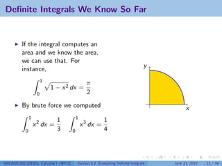
![The definite integral as a limit
Definition
If f is a function defined on [a, b], the definite integral of f from a to b
is the number
b n
f (x) dx = lim f (ci ) ∆x
a n→∞
i=1
b−a
where ∆x = , and for each i, xi = a + i∆x, and ci is a point in
n
[xi−1 , xi ].
Theorem
If f is continuous on [a, b] or if f has only finitely many jump
discontinuities, then f is integrable on [a, b]; that is, the definite integral
b
f (x) dx exists and is the same for any choice of ci .
a
V63.0121.002.2010Su, Calculus I (NYU) Section 5.3 Evaluating Definite Integrals June 21, 2010 6 / 44](https://image.slidesharecdn.com/lesson26-evaluatingdefiniteintegralsslides-100622161907-phpapp01/85/Lesson-26-Evaluating-Definite-Integrals-6-320.jpg)


![Example
1
4
Estimate dx using the midpoint rule and four divisions.
0 1 + x2
Solution
Dividing up [0, 1] into 4 pieces gives
1 2 3 4
x0 = 0, x1 = , x2 = , x3 = , x4 =
4 4 4 4
So the midpoint rule gives
1 4 4 4 4
M4 = 2
+ 2
+ 2
+
4 1 + (1/8) 1 + (3/8) 1 + (5/8) 1 + (7/8)2
V63.0121.002.2010Su, Calculus I (NYU) Section 5.3 Evaluating Definite Integrals June 21, 2010 8 / 44](https://image.slidesharecdn.com/lesson26-evaluatingdefiniteintegralsslides-100622161907-phpapp01/85/Lesson-26-Evaluating-Definite-Integrals-9-320.jpg)
![Example
1
4
Estimate dx using the midpoint rule and four divisions.
0 1 + x2
Solution
Dividing up [0, 1] into 4 pieces gives
1 2 3 4
x0 = 0, x1 = , x2 = , x3 = , x4 =
4 4 4 4
So the midpoint rule gives
1 4 4 4 4
M4 = 2
+ 2
+ 2
+
4 1 + (1/8) 1 + (3/8) 1 + (5/8) 1 + (7/8)2
1 4 4 4 4
= + + +
4 65/64 73/64 89/64 113/64
V63.0121.002.2010Su, Calculus I (NYU) Section 5.3 Evaluating Definite Integrals June 21, 2010 8 / 44](https://image.slidesharecdn.com/lesson26-evaluatingdefiniteintegralsslides-100622161907-phpapp01/85/Lesson-26-Evaluating-Definite-Integrals-10-320.jpg)
![Example
1
4
Estimate dx using the midpoint rule and four divisions.
0 1 + x2
Solution
Dividing up [0, 1] into 4 pieces gives
1 2 3 4
x0 = 0, x1 = , x2 = , x3 = , x4 =
4 4 4 4
So the midpoint rule gives
1 4 4 4 4
M4 = 2
+ 2
+ 2
+
4 1 + (1/8) 1 + (3/8) 1 + (5/8) 1 + (7/8)2
1 4 4 4 4
= + + +
4 65/64 73/64 89/64 113/64
150, 166, 784
= ≈ 3.1468
47, 720, 465
V63.0121.002.2010Su, Calculus I (NYU) Section 5.3 Evaluating Definite Integrals June 21, 2010 8 / 44](https://image.slidesharecdn.com/lesson26-evaluatingdefiniteintegralsslides-100622161907-phpapp01/85/Lesson-26-Evaluating-Definite-Integrals-11-320.jpg)
![Properties of the integral
Theorem (Additive Properties of the Integral)
Let f and g be integrable functions on [a, b] and c a constant. Then
b
1. c dx = c(b − a)
a
b b b
2. [f (x) + g (x)] dx = f (x) dx + g (x) dx.
a a a
b b
3. cf (x) dx = c f (x) dx.
a a
b b b
4. [f (x) − g (x)] dx = f (x) dx − g (x) dx.
a a a
V63.0121.002.2010Su, Calculus I (NYU) Section 5.3 Evaluating Definite Integrals June 21, 2010 9 / 44](https://image.slidesharecdn.com/lesson26-evaluatingdefiniteintegralsslides-100622161907-phpapp01/85/Lesson-26-Evaluating-Definite-Integrals-12-320.jpg)

![Comparison Properties of the Integral
Theorem
Let f and g be integrable functions on [a, b].
6. If f (x) ≥ 0 for all x in [a, b], then
b
f (x) dx ≥ 0
a
V63.0121.002.2010Su, Calculus I (NYU) Section 5.3 Evaluating Definite Integrals June 21, 2010 12 / 44](https://image.slidesharecdn.com/lesson26-evaluatingdefiniteintegralsslides-100622161907-phpapp01/85/Lesson-26-Evaluating-Definite-Integrals-15-320.jpg)
![Integral of a nonnegative function is nonnegative
Proof.
If f (x) ≥ 0 for all x in [a, b], then for any number of divisions n and choice
of sample points {ci }:
n n
Sn = f (ci ) ∆x ≥ 0 · ∆x = 0
i=1 ≥0 i=1
Since Sn ≥ 0 for all n, the limit of {Sn } is nonnegative, too:
b
f (x) dx = lim Sn ≥ 0
a n→∞
≥0
V63.0121.002.2010Su, Calculus I (NYU) Section 5.3 Evaluating Definite Integrals June 21, 2010 13 / 44](https://image.slidesharecdn.com/lesson26-evaluatingdefiniteintegralsslides-100622161907-phpapp01/85/Lesson-26-Evaluating-Definite-Integrals-16-320.jpg)
![Comparison Properties of the Integral
Theorem
Let f and g be integrable functions on [a, b].
6. If f (x) ≥ 0 for all x in [a, b], then
b
f (x) dx ≥ 0
a
7. If f (x) ≥ g (x) for all x in [a, b], then
b b
f (x) dx ≥ g (x) dx
a a
V63.0121.002.2010Su, Calculus I (NYU) Section 5.3 Evaluating Definite Integrals June 21, 2010 14 / 44](https://image.slidesharecdn.com/lesson26-evaluatingdefiniteintegralsslides-100622161907-phpapp01/85/Lesson-26-Evaluating-Definite-Integrals-17-320.jpg)
![The definite integral is “increasing”
Proof.
Let h(x) = f (x) − g (x). If f (x) ≥ g (x) for all x in [a, b], then h(x) ≥ 0
for all x in [a, b]. So by the previous property
b
h(x) dx ≥ 0
a
This means that
b b b b
f (x) dx − g (x) dx = (f (x) − g (x)) dx = h(x) dx ≥ 0
a a a a
So
b b
f (x) dx ≥ g (x) dx
a a
V63.0121.002.2010Su, Calculus I (NYU) Section 5.3 Evaluating Definite Integrals June 21, 2010 15 / 44](https://image.slidesharecdn.com/lesson26-evaluatingdefiniteintegralsslides-100622161907-phpapp01/85/Lesson-26-Evaluating-Definite-Integrals-18-320.jpg)
![Comparison Properties of the Integral
Theorem
Let f and g be integrable functions on [a, b].
6. If f (x) ≥ 0 for all x in [a, b], then
b
f (x) dx ≥ 0
a
7. If f (x) ≥ g (x) for all x in [a, b], then
b b
f (x) dx ≥ g (x) dx
a a
8. If m ≤ f (x) ≤ M for all x in [a, b], then
b
m(b − a) ≤ f (x) dx ≤ M(b − a)
a
V63.0121.002.2010Su, Calculus I (NYU) Section 5.3 Evaluating Definite Integrals June 21, 2010 16 / 44](https://image.slidesharecdn.com/lesson26-evaluatingdefiniteintegralsslides-100622161907-phpapp01/85/Lesson-26-Evaluating-Definite-Integrals-19-320.jpg)
![Bounding the integral using bounds of the function
Proof.
If m ≤ f (x) ≤ M on for all x in [a, b], then by the previous property
b b b
m dx ≤ f (x) dx ≤ M dx
a a a
By Property 1, the integral of a constant function is the product of the
constant and the width of the interval. So:
b
m(b − a) ≤ f (x) dx ≤ M(b − a)
a
V63.0121.002.2010Su, Calculus I (NYU) Section 5.3 Evaluating Definite Integrals June 21, 2010 17 / 44](https://image.slidesharecdn.com/lesson26-evaluatingdefiniteintegralsslides-100622161907-phpapp01/85/Lesson-26-Evaluating-Definite-Integrals-20-320.jpg)


![Theorem of the Day
Theorem (The Second Fundamental Theorem of Calculus)
Suppose f is integrable on [a, b] and f = F for another function F , then
b
f (x) dx = F (b) − F (a).
a
V63.0121.002.2010Su, Calculus I (NYU) Section 5.3 Evaluating Definite Integrals June 21, 2010 21 / 44](https://image.slidesharecdn.com/lesson26-evaluatingdefiniteintegralsslides-100622161907-phpapp01/85/Lesson-26-Evaluating-Definite-Integrals-25-320.jpg)
![Theorem of the Day
Theorem (The Second Fundamental Theorem of Calculus)
Suppose f is integrable on [a, b] and f = F for another function F , then
b
f (x) dx = F (b) − F (a).
a
Note
In Section 5.3, this theorem is called “The Evaluation Theorem”. Nobody
else in the world calls it that.
V63.0121.002.2010Su, Calculus I (NYU) Section 5.3 Evaluating Definite Integrals June 21, 2010 21 / 44](https://image.slidesharecdn.com/lesson26-evaluatingdefiniteintegralsslides-100622161907-phpapp01/85/Lesson-26-Evaluating-Definite-Integrals-26-320.jpg)
![Proving the Second FTC
b−a
Divide up [a, b] into n pieces of equal width ∆x = as usual. For
n
each i, F is continuous on [xi−1 , xi ] and differentiable on (xi−1 , xi ). So
there is a point ci in (xi−1 , xi ) with
F (xi ) − F (xi−1 )
= F (ci ) = f (ci )
xi − xi−1
Or
f (ci )∆x = F (xi ) − F (xi−1 )
V63.0121.002.2010Su, Calculus I (NYU) Section 5.3 Evaluating Definite Integrals June 21, 2010 22 / 44](https://image.slidesharecdn.com/lesson26-evaluatingdefiniteintegralsslides-100622161907-phpapp01/85/Lesson-26-Evaluating-Definite-Integrals-27-320.jpg)


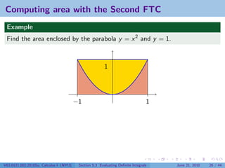
![Computing area with the Second FTC
Example
Find the area between y = x 3 and the x-axis, between x = 0 and x = 1.
Solution
1 1
x4 1
A= x 3 dx = =
0 4 0 4
Here we use the notation F (x)|b or [F (x)]b to mean F (b) − F (a).
a a
V63.0121.002.2010Su, Calculus I (NYU) Section 5.3 Evaluating Definite Integrals June 21, 2010 25 / 44](https://image.slidesharecdn.com/lesson26-evaluatingdefiniteintegralsslides-100622161907-phpapp01/85/Lesson-26-Evaluating-Definite-Integrals-33-320.jpg)


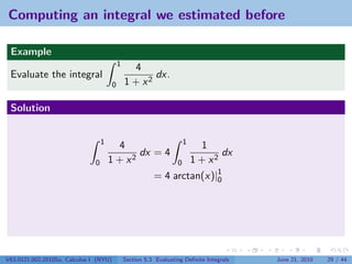
![Example
1
4
Estimate dx using the midpoint rule and four divisions.
0 1 + x2
Solution
Dividing up [0, 1] into 4 pieces gives
1 2 3 4
x0 = 0, x1 = , x2 = , x3 = , x4 =
4 4 4 4
So the midpoint rule gives
1 4 4 4 4
M4 = 2
+ 2
+ 2
+
4 1 + (1/8) 1 + (3/8) 1 + (5/8) 1 + (7/8)2
1 4 4 4 4
= + + +
4 65/64 73/64 89/64 113/64
150, 166, 784
= ≈ 3.1468
47, 720, 465
V63.0121.002.2010Su, Calculus I (NYU) Section 5.3 Evaluating Definite Integrals June 21, 2010 28 / 44](https://image.slidesharecdn.com/lesson26-evaluatingdefiniteintegralsslides-100622161907-phpapp01/85/Lesson-26-Evaluating-Definite-Integrals-38-320.jpg)


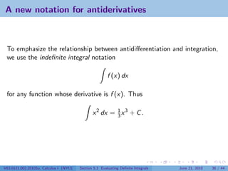
![My first table of integrals
[f (x) + g (x)] dx = f (x) dx + g (x) dx
x n+1
x n dx = + C (n = −1) cf (x) dx = c f (x) dx
n+1
1
e x dx = e x + C dx = ln |x| + C
x
ax
sin x dx = − cos x + C ax dx = +C
ln a
cos x dx = sin x + C csc2 x dx = − cot x + C
sec2 x dx = tan x + C csc x cot x dx = − csc x + C
1
sec x tan x dx = sec x + C √ dx = arcsin x + C
1 − x2
1
dx = arctan x + C
1 + x2
V63.0121.002.2010Su, Calculus I (NYU) Section 5.3 Evaluating Definite Integrals June 21, 2010 37 / 44](https://image.slidesharecdn.com/lesson26-evaluatingdefiniteintegralsslides-100622161907-phpapp01/85/Lesson-26-Evaluating-Definite-Integrals-58-320.jpg)


![Example
Find the area between the graph of y = (x − 1)(x − 2), the x-axis, and the
vertical lines x = 0 and x = 3.
Solution
3
Consider (x − 1)(x − 2) dx. Notice the integrand is positive on [0, 1)
0
and (2, 3], and negative on (1, 2).
V63.0121.002.2010Su, Calculus I (NYU) Section 5.3 Evaluating Definite Integrals June 21, 2010 41 / 44](https://image.slidesharecdn.com/lesson26-evaluatingdefiniteintegralsslides-100622161907-phpapp01/85/Lesson-26-Evaluating-Definite-Integrals-63-320.jpg)
![Example
Find the area between the graph of y = (x − 1)(x − 2), the x-axis, and the
vertical lines x = 0 and x = 3.
Solution
3
Consider (x − 1)(x − 2) dx. Notice the integrand is positive on [0, 1)
0
and (2, 3], and negative on (1, 2). If we want the area of the region, we
have to do
1 2 3
A= (x − 1)(x − 2) dx − (x − 1)(x − 2) dx + (x − 1)(x − 2) dx
0 1 2
1 3 1 2 3
= 3x − 2 x 2 + 2x
3
0
− 1 3
3x − 3 x 2 + 2x
2 1
+ 1 3
3x − 2 x 2 + 2x
3
2
5 1 5 11
= − − + = .
6 6 6 6
V63.0121.002.2010Su, Calculus I (NYU) Section 5.3 Evaluating Definite Integrals June 21, 2010 41 / 44](https://image.slidesharecdn.com/lesson26-evaluatingdefiniteintegralsslides-100622161907-phpapp01/85/Lesson-26-Evaluating-Definite-Integrals-64-320.jpg)


- The document is from a Calculus I class at New York University and covers evaluating definite integrals. - It discusses using the Evaluation Theorem to evaluate definite integrals, writing antiderivatives as indefinite integrals, and interpreting definite integrals as the net change of a function over an interval. - Examples are provided of using the midpoint rule to estimate a definite integral, and properties of definite integrals like additivity and comparison properties are reviewed.