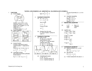
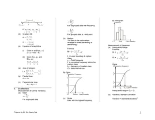
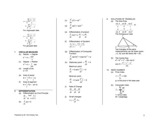
This document contains notes and formulae on additional mathematics for Form 4. It covers topics such as functions, quadratic equations, quadratic functions, indices and logarithms, coordinate geometry, statistics, circular measure, differentiation, solutions of triangles, and index numbers. The key points covered include the definition of functions, the formula for the sum and product of roots of a quadratic equation, the axis of symmetry and nature of roots of quadratic functions, and common differentiation rules.

1. NOTES AND FORMULAE ADDITIONAL MATHEMATICS FORM 4
1. FUNCTIONS 2 6 The axis of symmetry is x – p = 0 or
(a) Arrow Diagram fg(x) = f( )= 2 x=p
x x
(c) Quadratic inequalities
2. QUADRATIC EQUATION (x – a)(x – b)  0
2
(a) ax + bx + c = 0 Range x  a, x  b
2
x =  b  b  4ac (x – a)(x – b)  0
2a Range a  x  b
Sum of roots: 4. INDICES AND LOGARITHM
Domain = set A = {−2, 1, 2, 3}
b
Codomain = set B = {1, 4, 8, 9}    n
Range = set of images = {1, 4, 9} a (a) x=a  loga x = n
Object of 4 = −2, 2 Product of roots: Index Logarithm
Image of 3 = 9 c Form Form
2  
In function notation f : x  x a
(b) Types of Relation (b) Logrithm Law
(b) Equation from the roots: 1. logaxy = logax + logay
2
x - (sum of roots)x + product of 2. loga x = logax – logay
roots = 0 y
n
One-to-one One-to-many 3. loga x = n logax
3. QUADRATIC FUNCTION 4. loga a = 1
(a) Types of roots 5. loga 1 = 0
2
b - 4ac > 0  2 real and
6. loga b = log c b
distinct/different roots.
Many-to-one Many-to-many 2 log c a
b - 4ac = 0  2 real and equal
roots/two same roots. 7. loga b = 1
(c) Inverse Function 2
b - 4ac < 0  no real root. log b a
Function f maps set A to set B 2
-1 b - 4ac  0  got real roots.
Inverse function f maps set B to y y y
set A. 5. COORDINATE GEOMETRY
Given f(x) = ax + b, let y = ax + b (a) Distance between A(x1, y1) and
y b -1 xb B(x2, y2)
x= f :x 0 x
a a 0 AB = ( x 2  x1 ) 2  ( y 2  y1 ) 2
x
(d) Composite Function 0 x (b) Mid point AB
2 2 2
fg(x) means the function g followed b - 4ac > 0 b - 4ac = 0 b - 4ac < 0 M  x1  x 2 , y1  y 2 
by the function f.  
 2 2 
2 (b) Completing the square
E.g. f : x  3x – 2, g : x  2 (c) P which divides AB in the ratio m : n
x y = a(x - p) + q
a +ve  minimum point (p, q)
a –ve  maximum point(p, q)
Prepared by Mr. Sim Kwang Yaw 1

2. m : n By Histogram :
x
 fx Frequency
P B(x2 , y2 )
f
A(x 1 , y1 )
For ungrouped data with frequency.
P  nx1  mx 2 ny1  my 2   fx
 ,  x
i
 nm nm  f
(d) Gradient AB For grouped data, xi = mid-point
m = y 2  y1
x 2  x1 (b) Median
The data in the centre when 0 Mode Class boundary
m =  y-intercept arranged in order (ascending or
x-intercept descending).
(e) Equation of straight line Measurement of Dispersion
(a) Interquartile Range
Formula Formula :
(i) Given m and A(x1, y1) 1
nF 1
M=L+ 2
C Q1 = L  4 n  F1  C
y – y1 = m(x – x1)
fm 1
f Q1
(ii) Given A(x1, y1) and L = Lower boundary of median 3
class. Q3 = L  4 n  F3  C
B(x2, y2) 3
f Q3
n = Total frequency
y  y1 y 2  y1
 F = cumulative frequency before the
x  x1 x 2  x1 median class Ogive :
fm = frequency of median class Cumulative frequency
(a) Area of polygon C = class interval size
L = 1 x1 x2 x3 ......... x1
By Ogive 3
__
2 y1 y 2 y 3 y1 Cumulative Frequency 4
n
(g) Parallel lines
m1 = m2 n
1
__ n
(h) Perpendicular lines 4
m1  m2 = -1. n
__
2
0 Q Q 3 Upper boundary
6. STATISTICS 1
Measurement of Central Tendency Interquartile range = Q3 – Q1
(a) Mean
0 Median Upper boundary (b) Variance, Standard Deviation
x
x
n 2
(c) Mode Variance = (standard deviation)
For ungrouped data
Data with the highest frequency
Prepared by Mr. Sim Kwang Yaw 2

3. 2 d (xn) = nxn-1 9. SOLUTIONS OF TRIANGLES
 
 ( x  x) (c) (a) The Sine Rule
n dx
sin A sin B sin C
d (axn) = anxn-1   , or,
=  x2 x
2 (d) a b c
n dx
a b c
For ungrouped data  
(e) Differentiation of product sin A sin B sin C
2 d (uv) = u dv + v du The Ambiguous Case
 
 f ( x  x)
dx dx dx
f
2
=  fx  x 2
(f) Differentiation of Quotient
f d  u  v du  u dv
For grouped data    dx 2 dx
dx  v  v
Two triangles of the same
7. CIRCULAR MEASURE (g) Differentiation of Composite measurements can be drawn given
(b) Radian  Degree Function C, AC and AB where AB < AC.
0 d (ax+b)n = n(ax+b)n-1 × a
 =   180
r
dx (b) The Cosine Rue
 2 2 2
a = b + c – 2bc cos A
(c) Degree  Radian (h) Stationary point 
dy = 0
b 2  c2  a 2
 =    rad cos A =
o
dx
180 Maximum point: 2bc
(d) Length of arc dy = 0 and d 2 y < 0
s = r 10. INDEX NUMBER
dx dx 2 (a) Price Index
(e) Area of sector p1
2
Minimum point: I  100
A = 1 r  = 1 rs 2 po
2 2 dy = 0 and d y > 0
p0 is the price in the base year.
(f) Area of segment dx dx 2
2
A = 1 r ( – sin ) (b) Composite Index
2 (i) Rate of Change
dy dy dx
  I
 IW
8. DIFFERENTIATION
(a) Differentiation by First Principle
dt dx dt W
dy had  y I = price index
 (j) Small changes: W = weightage
dx x  0  x dy
d (a) = 0  y  . x
(b) dx
dx
Prepared by Mr. Sim Kwang Yaw 3