This document summarizes a calculus lecture on the Mean Value Theorem. It begins with announcements about exams and assignments. It then outlines the topics to be covered: Rolle's Theorem and the Mean Value Theorem, applications of the MVT, and why the MVT is important. It provides heuristic motivations and mathematical statements of Rolle's Theorem and the Mean Value Theorem. It also includes a proof of the Mean Value Theorem using Rolle's Theorem.

1. Section 4.2
The Mean Value Theorem
V63.0121.002.2010Su, Calculus I
New York University
June 8, 2010
Announcements
Exams not graded yet
Assignment 4 is on the website
Quiz 3 on Thursday covering 3.3, 3.4, 3.5, 3.7

2. Announcements
Exams not graded yet
Assignment 4 is on the
website
Quiz 3 on Thursday covering
3.3, 3.4, 3.5, 3.7
V63.0121.002.2010Su, Calculus I (NYU) Section 4.2 The Mean Value Theorem June 8, 2010 2 / 28

3. Objectives
Understand and be able to
explain the statement of
Rolle’s Theorem.
Understand and be able to
explain the statement of the
Mean Value Theorem.
V63.0121.002.2010Su, Calculus I (NYU) Section 4.2 The Mean Value Theorem June 8, 2010 3 / 28

4. Outline
Rolle’s Theorem
The Mean Value Theorem
Applications
Why the MVT is the MITC
Functions with derivatives that are zero
MVT and differentiability
V63.0121.002.2010Su, Calculus I (NYU) Section 4.2 The Mean Value Theorem June 8, 2010 4 / 28

5. Heuristic Motivation for Rolle’s Theorem
If you bike up a hill, then back down, at some point your elevation was
stationary.
Image credit: SpringSun
V63.0121.002.2010Su, Calculus I (NYU) Section 4.2 The Mean Value Theorem June 8, 2010 5 / 28

6. Mathematical Statement of Rolle’s Theorem
Theorem (Rolle’s Theorem)
Let f be continuous on [a, b]
and differentiable on (a, b).
Suppose f (a) = f (b). Then
there exists a point c in (a, b)
such that f (c) = 0.
a b

7. Mathematical Statement of Rolle’s Theorem
Theorem (Rolle’s Theorem)
c
Let f be continuous on [a, b]
and differentiable on (a, b).
Suppose f (a) = f (b). Then
there exists a point c in (a, b)
such that f (c) = 0.
a b
V63.0121.002.2010Su, Calculus I (NYU) Section 4.2 The Mean Value Theorem June 8, 2010 6 / 28

8. Flowchart proof of Rolle’s Theorem
endpoints
Let c be Let d be
are max
the max pt the min pt
and min
f is
is c an is d an
yes yes constant
endpoint? endpoint?
on [a, b]
no no
f (x) ≡ 0
f (c) = 0 f (d) = 0
on (a, b)
V63.0121.002.2010Su, Calculus I (NYU) Section 4.2 The Mean Value Theorem June 8, 2010 8 / 28

9. Outline
Rolle’s Theorem
The Mean Value Theorem
Applications
Why the MVT is the MITC
Functions with derivatives that are zero
MVT and differentiability
V63.0121.002.2010Su, Calculus I (NYU) Section 4.2 The Mean Value Theorem June 8, 2010 9 / 28

10. Heuristic Motivation for The Mean Value Theorem
If you drive between points A and B, at some time your speedometer
reading was the same as your average speed over the drive.
Image credit: ClintJCL
V63.0121.002.2010Su, Calculus I (NYU) Section 4.2 The Mean Value Theorem June 8, 2010 10 / 28

11. The Mean Value Theorem
Theorem (The Mean Value Theorem)
Let f be continuous on [a, b]
and differentiable on (a, b).
Then there exists a point c in
(a, b) such that
f (b) − f (a) b
= f (c).
b−a
a

12. The Mean Value Theorem
Theorem (The Mean Value Theorem)
Let f be continuous on [a, b]
and differentiable on (a, b).
Then there exists a point c in
(a, b) such that
f (b) − f (a) b
= f (c).
b−a
a

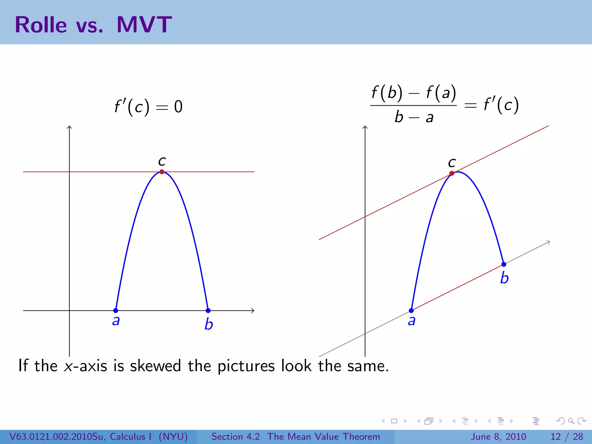
13. The Mean Value Theorem
Theorem (The Mean Value Theorem)
c
Let f be continuous on [a, b]
and differentiable on (a, b).
Then there exists a point c in
(a, b) such that
f (b) − f (a) b
= f (c).
b−a
a
V63.0121.002.2010Su, Calculus I (NYU) Section 4.2 The Mean Value Theorem June 8, 2010 11 / 28

14. Rolle vs. MVT
f (b) − f (a)
f (c) = 0 = f (c)
b−a
c c
b
a b a
V63.0121.002.2010Su, Calculus I (NYU) Section 4.2 The Mean Value Theorem June 8, 2010 12 / 28

15. Rolle vs. MVT
f (b) − f (a)
f (c) = 0 = f (c)
b−a
c c
b
a b a
If the x-axis is skewed the pictures look the same.
V63.0121.002.2010Su, Calculus I (NYU) Section 4.2 The Mean Value Theorem June 8, 2010 12 / 28

16. Proof of the Mean Value Theorem
Proof.
The line connecting (a, f (a)) and (b, f (b)) has equation
f (b) − f (a)
y − f (a) = (x − a)
b−a
V63.0121.002.2010Su, Calculus I (NYU) Section 4.2 The Mean Value Theorem June 8, 2010 13 / 28

17. Proof of the Mean Value Theorem
Proof.
The line connecting (a, f (a)) and (b, f (b)) has equation
f (b) − f (a)
y − f (a) = (x − a)
b−a
Apply Rolle’s Theorem to the function
f (b) − f (a)
g (x) = f (x) − f (a) − (x − a).
b−a
V63.0121.002.2010Su, Calculus I (NYU) Section 4.2 The Mean Value Theorem June 8, 2010 13 / 28

18. Proof of the Mean Value Theorem
Proof.
The line connecting (a, f (a)) and (b, f (b)) has equation
f (b) − f (a)
y − f (a) = (x − a)
b−a
Apply Rolle’s Theorem to the function
f (b) − f (a)
g (x) = f (x) − f (a) − (x − a).
b−a
Then g is continuous on [a, b] and differentiable on (a, b) since f is.
V63.0121.002.2010Su, Calculus I (NYU) Section 4.2 The Mean Value Theorem June 8, 2010 13 / 28

19. Proof of the Mean Value Theorem
Proof.
The line connecting (a, f (a)) and (b, f (b)) has equation
f (b) − f (a)
y − f (a) = (x − a)
b−a
Apply Rolle’s Theorem to the function
f (b) − f (a)
g (x) = f (x) − f (a) − (x − a).
b−a
Then g is continuous on [a, b] and differentiable on (a, b) since f is. Also
g (a) = 0 and g (b) = 0 (check both)
V63.0121.002.2010Su, Calculus I (NYU) Section 4.2 The Mean Value Theorem June 8, 2010 13 / 28

20. Proof of the Mean Value Theorem
Proof.
The line connecting (a, f (a)) and (b, f (b)) has equation
f (b) − f (a)
y − f (a) = (x − a)
b−a
Apply Rolle’s Theorem to the function
f (b) − f (a)
g (x) = f (x) − f (a) − (x − a).
b−a
Then g is continuous on [a, b] and differentiable on (a, b) since f is. Also
g (a) = 0 and g (b) = 0 (check both) So by Rolle’s Theorem there exists a
point c in (a, b) such that
f (b) − f (a)
0 = g (c) = f (c) − .
b−a
V63.0121.002.2010Su, Calculus I (NYU) Section 4.2 The Mean Value Theorem June 8, 2010 13 / 28

21. Using the MVT to count solutions
Example
Show that there is a unique solution to the equation x 3 − x = 100 in the
interval [4, 5].
V63.0121.002.2010Su, Calculus I (NYU) Section 4.2 The Mean Value Theorem June 8, 2010 14 / 28

22. Using the MVT to count solutions
Example
Show that there is a unique solution to the equation x 3 − x = 100 in the
interval [4, 5].
Solution
By the Intermediate Value Theorem, the function f (x) = x 3 − x must
take the value 100 at some point on c in (4, 5).
V63.0121.002.2010Su, Calculus I (NYU) Section 4.2 The Mean Value Theorem June 8, 2010 14 / 28

23. Using the MVT to count solutions
Example
Show that there is a unique solution to the equation x 3 − x = 100 in the
interval [4, 5].
Solution
By the Intermediate Value Theorem, the function f (x) = x 3 − x must
take the value 100 at some point on c in (4, 5).
If there were two points c1 and c2 with f (c1 ) = f (c2 ) = 100, then
somewhere between them would be a point c3 between them with
f (c3 ) = 0.
V63.0121.002.2010Su, Calculus I (NYU) Section 4.2 The Mean Value Theorem June 8, 2010 14 / 28

24. Using the MVT to count solutions
Example
Show that there is a unique solution to the equation x 3 − x = 100 in the
interval [4, 5].
Solution
By the Intermediate Value Theorem, the function f (x) = x 3 − x must
take the value 100 at some point on c in (4, 5).
If there were two points c1 and c2 with f (c1 ) = f (c2 ) = 100, then
somewhere between them would be a point c3 between them with
f (c3 ) = 0.
However, f (x) = 3x 2 − 1, which is positive all along (4, 5). So this is
impossible.
V63.0121.002.2010Su, Calculus I (NYU) Section 4.2 The Mean Value Theorem June 8, 2010 14 / 28

25. Using the MVT to estimate
Example
We know that |sin x| ≤ 1 for all x. Show that |sin x| ≤ |x|.
V63.0121.002.2010Su, Calculus I (NYU) Section 4.2 The Mean Value Theorem June 8, 2010 15 / 28

26. Using the MVT to estimate
Example
We know that |sin x| ≤ 1 for all x. Show that |sin x| ≤ |x|.
Solution
Apply the MVT to the function f (t) = sin t on [0, x]. We get
sin x − sin 0
= cos(c)
x −0
for some c in (0, x). Since |cos(c)| ≤ 1, we get
sin x
≤ 1 =⇒ |sin x| ≤ |x|
x
V63.0121.002.2010Su, Calculus I (NYU) Section 4.2 The Mean Value Theorem June 8, 2010 15 / 28

27. Using the MVT to estimate II
Example
Let f be a differentiable function with f (1) = 3 and f (x) < 2 for all x in
[0, 5]. Could f (4) ≥ 9?
V63.0121.002.2010Su, Calculus I (NYU) Section 4.2 The Mean Value Theorem June 8, 2010 16 / 28

28. Using the MVT to estimate II
Example
Let f be a differentiable function with f (1) = 3 and f (x) < 2 for all x in
[0, 5]. Could f (4) ≥ 9?
Solution
y (4, 9)
By MVT
f (4) − f (1) (4, f (4))
= f (c) < 2
4−1
for some c in (1, 4). Therefore
f (4) = f (1) + f (c)(3) < 3 + 2 · 3 = 9.
(1, 3)
So no, it is impossible that f (4) ≥ 9.
x
V63.0121.002.2010Su, Calculus I (NYU) Section 4.2 The Mean Value Theorem June 8, 2010 16 / 28

29. Food for Thought
Question
A driver travels along the New Jersey Turnpike using E-ZPass. The system
takes note of the time and place the driver enters and exits the Turnpike.
A week after his trip, the driver gets a speeding ticket in the mail. Which
of the following best describes the situation?
(a) E-ZPass cannot prove that the driver was speeding
(b) E-ZPass can prove that the driver was speeding
(c) The driver’s actual maximum speed exceeds his ticketed speed
(d) Both (b) and (c).
V63.0121.002.2010Su, Calculus I (NYU) Section 4.2 The Mean Value Theorem June 8, 2010 17 / 28

30. Food for Thought
Question
A driver travels along the New Jersey Turnpike using E-ZPass. The system
takes note of the time and place the driver enters and exits the Turnpike.
A week after his trip, the driver gets a speeding ticket in the mail. Which
of the following best describes the situation?
(a) E-ZPass cannot prove that the driver was speeding
(b) E-ZPass can prove that the driver was speeding
(c) The driver’s actual maximum speed exceeds his ticketed speed
(d) Both (b) and (c).
V63.0121.002.2010Su, Calculus I (NYU) Section 4.2 The Mean Value Theorem June 8, 2010 17 / 28

31. Outline
Rolle’s Theorem
The Mean Value Theorem
Applications
Why the MVT is the MITC
Functions with derivatives that are zero
MVT and differentiability
V63.0121.002.2010Su, Calculus I (NYU) Section 4.2 The Mean Value Theorem June 8, 2010 18 / 28

32. Functions with derivatives that are zero
Fact
If f is constant on (a, b), then f (x) = 0 on (a, b).
V63.0121.002.2010Su, Calculus I (NYU) Section 4.2 The Mean Value Theorem June 8, 2010 19 / 28

33. Functions with derivatives that are zero
Fact
If f is constant on (a, b), then f (x) = 0 on (a, b).
The limit of difference quotients must be 0
The tangent line to a line is that line, and a constant function’s graph
is a horizontal line, which has slope 0.
Implied by the power rule since c = cx 0
V63.0121.002.2010Su, Calculus I (NYU) Section 4.2 The Mean Value Theorem June 8, 2010 19 / 28

34. Functions with derivatives that are zero
Fact
If f is constant on (a, b), then f (x) = 0 on (a, b).
The limit of difference quotients must be 0
The tangent line to a line is that line, and a constant function’s graph
is a horizontal line, which has slope 0.
Implied by the power rule since c = cx 0
Question
If f (x) = 0 is f necessarily a constant function?
V63.0121.002.2010Su, Calculus I (NYU) Section 4.2 The Mean Value Theorem June 8, 2010 19 / 28

35. Functions with derivatives that are zero
Fact
If f is constant on (a, b), then f (x) = 0 on (a, b).
The limit of difference quotients must be 0
The tangent line to a line is that line, and a constant function’s graph
is a horizontal line, which has slope 0.
Implied by the power rule since c = cx 0
Question
If f (x) = 0 is f necessarily a constant function?
It seems true
But so far no theorem (that we have proven) uses information about
the derivative of a function to determine information about the
function itself
V63.0121.002.2010Su, Calculus I (NYU) Section 4.2 The Mean Value Theorem June 8, 2010 19 / 28

36. Why the MVT is the MITC
Most Important Theorem In Calculus!
Theorem
Let f = 0 on an interval (a, b).
V63.0121.002.2010Su, Calculus I (NYU) Section 4.2 The Mean Value Theorem June 8, 2010 20 / 28

37. Why the MVT is the MITC
Most Important Theorem In Calculus!
Theorem
Let f = 0 on an interval (a, b). Then f is constant on (a, b).
V63.0121.002.2010Su, Calculus I (NYU) Section 4.2 The Mean Value Theorem June 8, 2010 20 / 28

38. Why the MVT is the MITC
Most Important Theorem In Calculus!
Theorem
Let f = 0 on an interval (a, b). Then f is constant on (a, b).
Proof.
Pick any points x and y in (a, b) with x < y . Then f is continuous on
[x, y ] and differentiable on (x, y ). By MVT there exists a point z in (x, y )
such that
f (y ) − f (x)
= f (z) = 0.
y −x
So f (y ) = f (x). Since this is true for all x and y in (a, b), then f is
constant.
V63.0121.002.2010Su, Calculus I (NYU) Section 4.2 The Mean Value Theorem June 8, 2010 20 / 28

39. Functions with the same derivative
Theorem
Suppose f and g are two differentiable functions on (a, b) with f = g .
Then f and g differ by a constant. That is, there exists a constant C such
that f (x) = g (x) + C .
V63.0121.002.2010Su, Calculus I (NYU) Section 4.2 The Mean Value Theorem June 8, 2010 21 / 28

40. Functions with the same derivative
Theorem
Suppose f and g are two differentiable functions on (a, b) with f = g .
Then f and g differ by a constant. That is, there exists a constant C such
that f (x) = g (x) + C .
Proof.
Let h(x) = f (x) − g (x)
Then h (x) = f (x) − g (x) = 0 on (a, b)
So h(x) = C , a constant
This means f (x) − g (x) = C on (a, b)
V63.0121.002.2010Su, Calculus I (NYU) Section 4.2 The Mean Value Theorem June 8, 2010 21 / 28

41. MVT and differentiability
Example
Let
−x if x ≤ 0
f (x) =
x2 if x ≥ 0
Is f differentiable at 0?
V63.0121.002.2010Su, Calculus I (NYU) Section 4.2 The Mean Value Theorem June 8, 2010 22 / 28

42. MVT and differentiability
Example
Let
−x if x ≤ 0
f (x) =
x2 if x ≥ 0
Is f differentiable at 0?
Solution (from the definition)
We have
f (x) − f (0) −x
lim = lim = −1
x→0− x −0 x→0 − x
f (x) − f (0) x2
lim+ = lim+ = lim+ x = 0
x→0 x −0 x→0 x x→0
Since these limits disagree, f is not differentiable at 0.
V63.0121.002.2010Su, Calculus I (NYU) Section 4.2 The Mean Value Theorem June 8, 2010 22 / 28

43. MVT and differentiability
Example
Let
−x if x ≤ 0
f (x) =
x2 if x ≥ 0
Is f differentiable at 0?
Solution (Sort of)
If x < 0, then f (x) = −1. If x > 0, then f (x) = 2x. Since
lim f (x) = 0 and lim f (x) = −1,
x→0+ x→0−
the limit lim f (x) does not exist and so f is not differentiable at 0.
x→0
V63.0121.002.2010Su, Calculus I (NYU) Section 4.2 The Mean Value Theorem June 8, 2010 22 / 28

44. Why only “sort of”?
f (x)
This solution is valid but less y f (x)
direct.
We seem to be using the
following fact: If lim f (x)
x→a
does not exist, then f is not
x
differentiable at a.
equivalently: If f is
differentiable at a, then
lim f (x) exists.
x→a
But this “fact” is not true!
V63.0121.002.2010Su, Calculus I (NYU) Section 4.2 The Mean Value Theorem June 8, 2010 23 / 28

45. Differentiable with discontinuous derivative
It is possible for a function f to be differentiable at a even if lim f (x)
x→a
does not exist.
Example
x 2 sin(1/x) if x = 0
Let f (x) = . Then when x = 0,
0 if x = 0
f (x) = 2x sin(1/x) + x 2 cos(1/x)(−1/x 2 ) = 2x sin(1/x) − cos(1/x),
which has no limit at 0. However,
f (x) − f (0) x 2 sin(1/x)
f (0) = lim = lim = lim x sin(1/x) = 0
x→0 x −0 x→0 x x→0
So f (0) = 0. Hence f is differentiable for all x, but f is not continuous at
0!
V63.0121.002.2010Su, Calculus I (NYU) Section 4.2 The Mean Value Theorem June 8, 2010 24 / 28

46. Differentiability FAIL
f (x) f (x)
x x
This function is differentiable at But the derivative is not
0. continuous at 0!
V63.0121.002.2010Su, Calculus I (NYU) Section 4.2 The Mean Value Theorem June 8, 2010 25 / 28

47. MVT to the rescue
Lemma
Suppose f is continuous on [a, b] and lim+ f (x) = m. Then
x→a
f (x) − f (a)
lim+ = m.
x→a x −a
V63.0121.002.2010Su, Calculus I (NYU) Section 4.2 The Mean Value Theorem June 8, 2010 26 / 28

48. MVT to the rescue
Lemma
Suppose f is continuous on [a, b] and lim+ f (x) = m. Then
x→a
f (x) − f (a)
lim+ = m.
x→a x −a
Proof.
Choose x near a and greater than a. Then
f (x) − f (a)
= f (cx )
x −a
for some cx where a < cx < x. As x → a, cx → a as well, so:
f (x) − f (a)
lim = lim+ f (cx ) = lim+ f (x) = m.
x→a+ x −a x→a x→a
V63.0121.002.2010Su, Calculus I (NYU) Section 4.2 The Mean Value Theorem June 8, 2010 26 / 28

49. Theorem
Suppose
lim f (x) = m1 and lim+ f (x) = m2
x→a− x→a
If m1 = m2 , then f is differentiable at a. If m1 = m2 , then f is not
differentiable at a.
V63.0121.002.2010Su, Calculus I (NYU) Section 4.2 The Mean Value Theorem June 8, 2010 27 / 28

50. Theorem
Suppose
lim f (x) = m1 and lim+ f (x) = m2
x→a− x→a
If m1 = m2 , then f is differentiable at a. If m1 = m2 , then f is not
differentiable at a.
Proof.
We know by the lemma that
f (x) − f (a)
lim = lim f (x)
x→a− x −a x→a−
f (x) − f (a)
lim+ = lim+ f (x)
x→a x −a x→a
The two-sided limit exists if (and only if) the two right-hand sides
agree.
V63.0121.002.2010Su, Calculus I (NYU) Section 4.2 The Mean Value Theorem June 8, 2010 27 / 28

51. Summary
Rolle’s Theorem: under suitable conditions, functions must have
critical points.
Mean Value Theorem: under suitable conditions, functions must have
an instantaneous rate of change equal to the average rate of change.
A function whose derivative is identically zero on an interval must be
constant on that interval.
E-ZPass is kinder than we realized.
V63.0121.002.2010Su, Calculus I (NYU) Section 4.2 The Mean Value Theorem June 8, 2010 28 / 28