Lesson 19: Curve Sketching

Section 4.4
Curve Sketching

V63.0121.006/016, Calculus I

New York University

April 1, 2010

. . . . . .

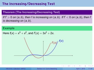
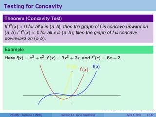
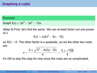
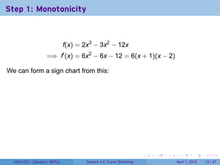
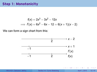
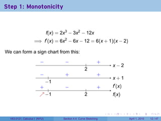
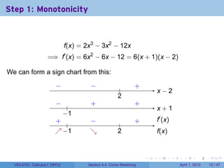
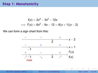
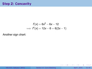
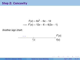
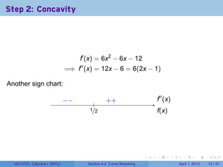
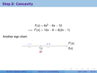
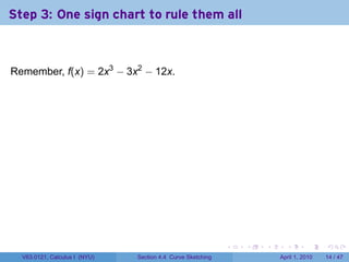
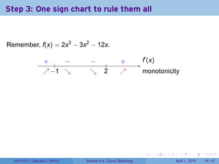
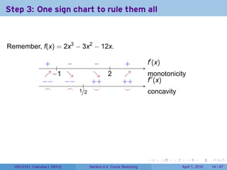
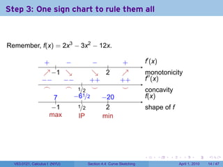
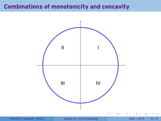
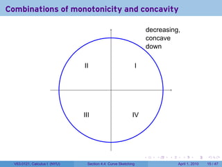
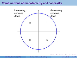
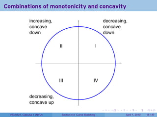
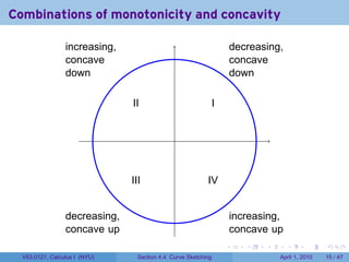
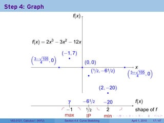
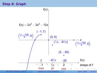
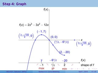
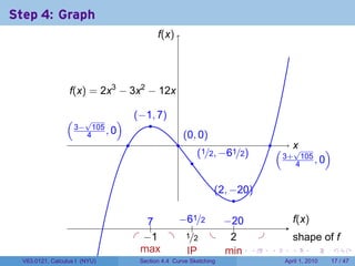
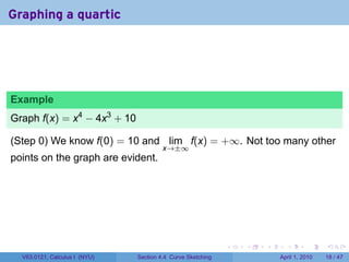
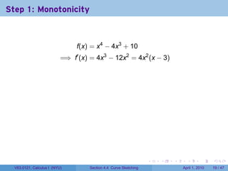
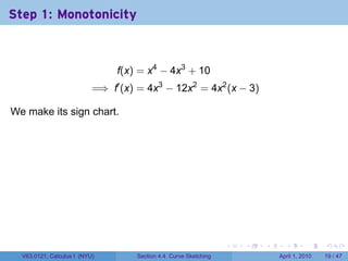
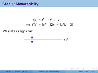
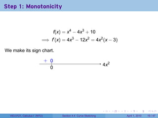
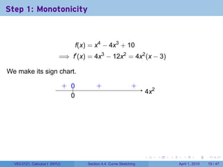
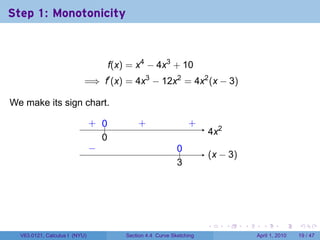
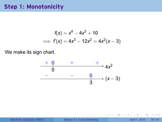
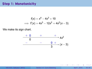
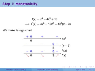
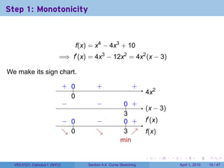
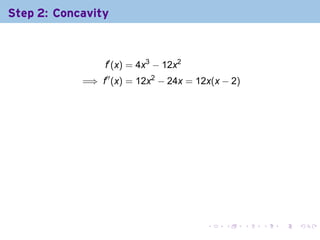
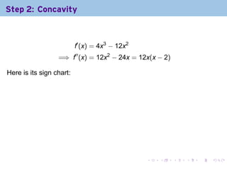
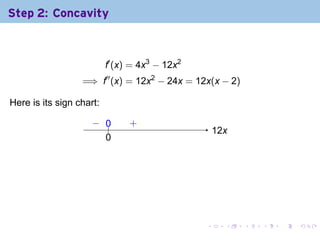
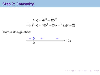
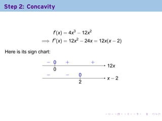
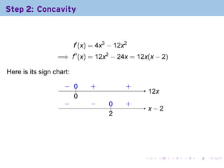
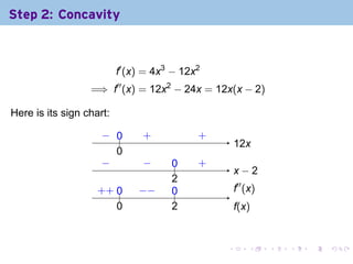
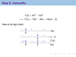
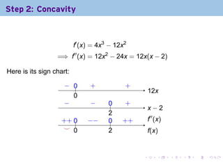
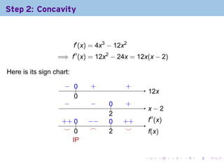
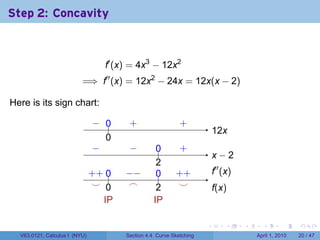
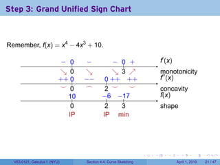
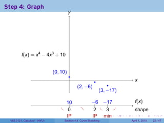
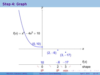
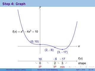
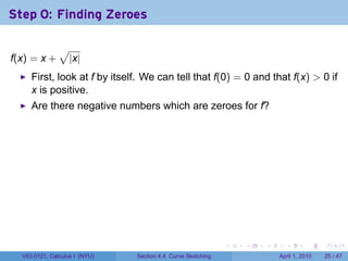
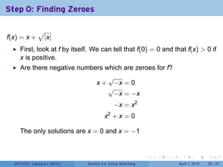
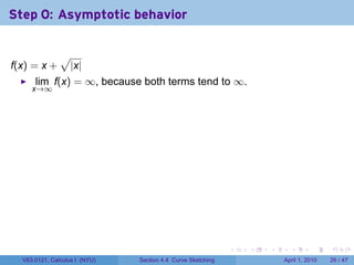
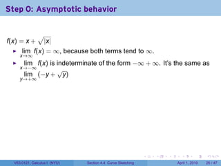
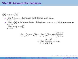
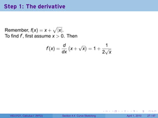
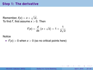
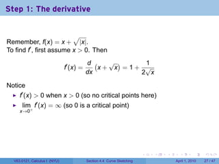
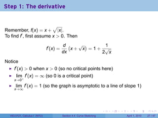
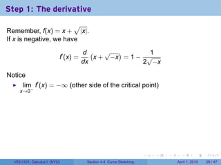
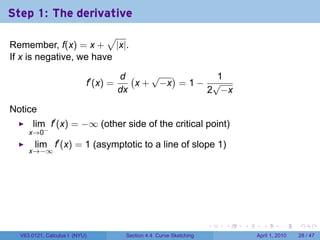
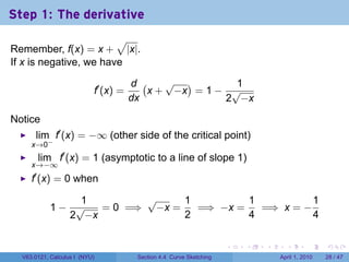
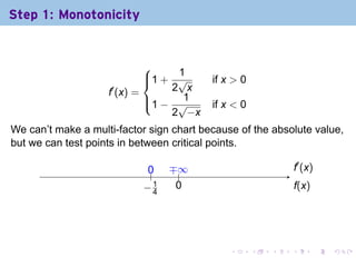
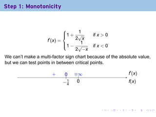
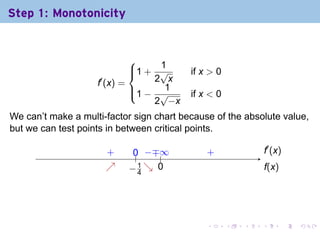
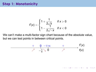
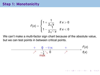
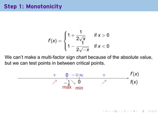
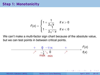
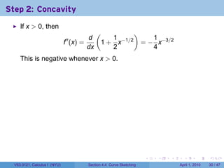
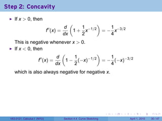
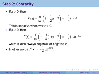
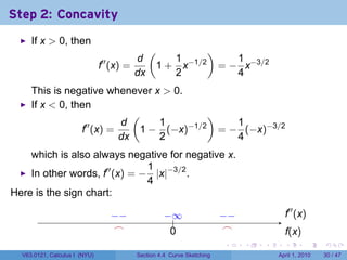
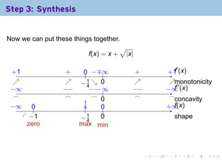
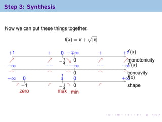
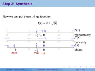
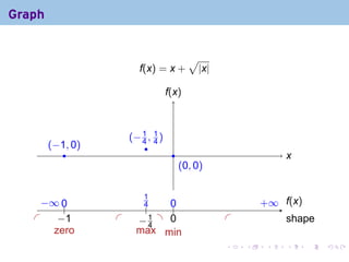
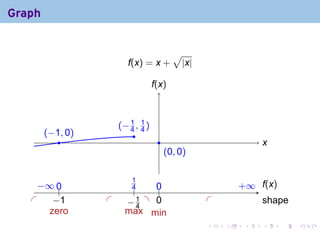
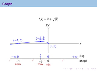
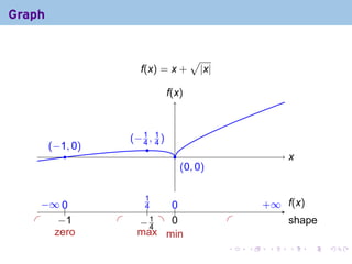
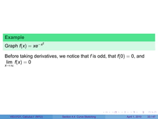
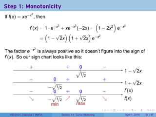
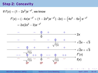
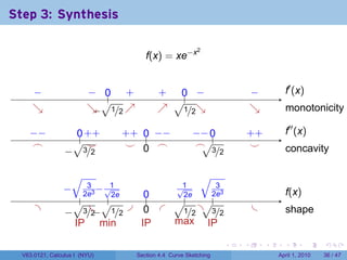
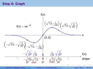
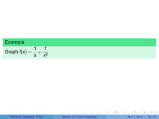
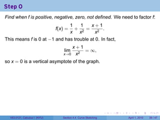
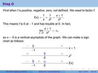
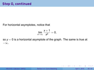
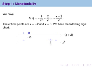
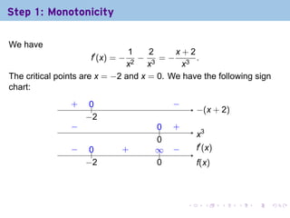
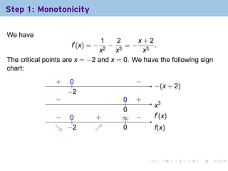
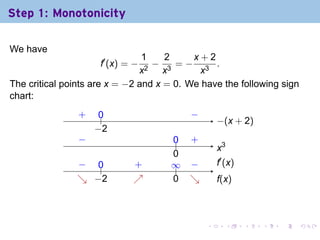
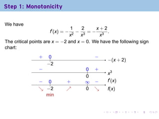
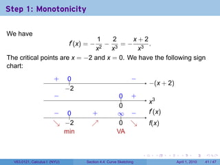
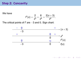
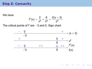
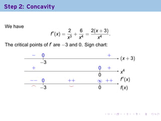
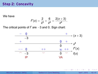
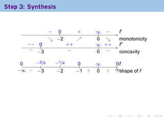
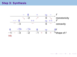
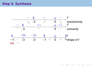
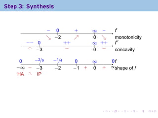
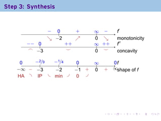
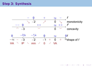
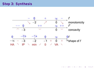
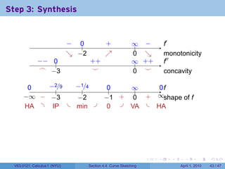
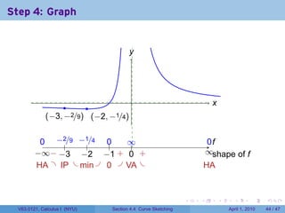
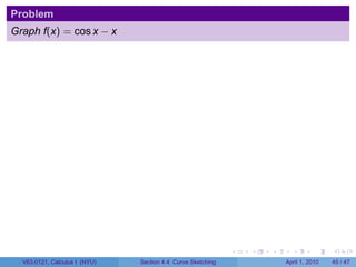
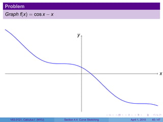
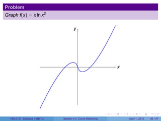
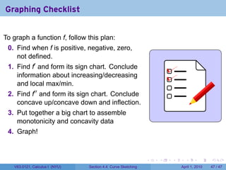
Second-chance Midterm: Tomorrow in Recitation

12 free-response questions, no multiple choice
Covers all sections so far, through today
Your score on this exam will replace your midterm score

. . . . . .

V63.0121, Calculus I (NYU) Section 4.4 Curve Sketching April 1, 2010 2 / 47

. . . . . .


Quiz 3 tomorrow in recitation

Section 2.6: implicit differentiation
Section 2.8: linear approximation and differentials
Section 3.1: exponential functions
Section 3.2: logarithms
Section 3.3: derivatives of logarithmic and exponential functions
Section 3.4: exponential growth and decay
Section 3.5: inverse trigonometric functions

. . . . . .


Outline

The Procedure

Simple examples
A cubic function
A quartic function

More Examples
Points of nondifferentiability
Horizontal asymptotes
Vertical asymptotes
Trigonometric and polynomial together
Logarithmic

. . . . . .


Objective

Given a function, graph it
completely, indicating
zeroes
asymptotes if applicable
critical points
local/global max/min
inflection points

. . . . . .


The Increasing/Decreasing Test

Theorem (The Increasing/Decreasing Test)
If f′ > 0 on (a, b), then f is increasing on (a, b). If f′ < 0 on (a, b), then f
is decreasing on (a, b).

Example
Here f(x) = x3 + x2 , and f′ (x) = 3x2 + 2x.

f
.(x)
.′ (x)
f

.

. . . . . .


Testing for Concavity
Theorem (Concavity Test)
If f′′ (x) > 0 for all x in (a, b), then the graph of f is concave upward on
(a, b) If f′′ (x) < 0 for all x in (a, b), then the graph of f is concave
downward on (a, b).

Example
Here f(x) = x3 + x2 , f′ (x) = 3x2 + 2x, and f′′ (x) = 6x + 2.
.′′ (x)
f f
.(x)
.′ (x)
f

.

. . . . . .


Graphing Checklist

To graph a function f, follow this plan:
0. Find when f is positive, negative, zero,
not defined.
1. Find f′ and form its sign chart. Conclude
information about increasing/decreasing
and local max/min.
2. Find f′′ and form its sign chart. Conclude
concave up/concave down and inflection.
3. Put together a big chart to assemble
monotonicity and concavity data
4. Graph!

. . . . . .


Outline

The Procedure

Simple examples
A cubic function
A quartic function

More Examples
Points of nondifferentiability
Horizontal asymptotes
Vertical asymptotes
Trigonometric and polynomial together
Logarithmic

. . . . . .


Graphing a cubic

Example
Graph f(x) = 2x3 − 3x2 − 12x.

. . . . . .


Graphing a cubic

Example
Graph f(x) = 2x3 − 3x2 − 12x.

(Step 0) First, let’s find the zeros. We can at least factor out one power
of x:
f(x) = x(2x2 − 3x − 12)
so f(0) = 0. The other factor is a quadratic, so we the other two roots
are √
√
3 ± 32 − 4(2)(−12) 3 ± 105
x= =
4 4
It’s OK to skip this step for now since the roots are so complicated.

. . . . . .


Step 1: Monotonicity

f(x) = 2x3 − 3x2 − 12x
=⇒ f′ (x) = 6x2 − 6x − 12 = 6(x + 1)(x − 2)

We can form a sign chart from this:

.

. . . . . .



f(x) = 2x3 − 3x2 − 12x
=⇒ f′ (x) = 6x2 − 6x − 12 = 6(x + 1)(x − 2)


. . . −2
x
2
.
. x
. +1
−
. 1
.′ (x)
f
. .
−
. 1 2
. f
.(x)

. . . . . .



f(x) = 2x3 − 3x2 − 12x
=⇒ f′ (x) = 6x2 − 6x − 12 = 6(x + 1)(x − 2)


−
. −
. . . .
+
. −2
x
2
.
. x
. +1
−
. 1
.′ (x)
f
. .
−
. 1 2
. f
.(x)

. . . . . .



f(x) = 2x3 − 3x2 − 12x
=⇒ f′ (x) = 6x2 − 6x − 12 = 6(x + 1)(x − 2)


−
. −
. . . .
+
. −2
x
2
.
−
. . .
+ .
+
x
. +1
−
. 1
.′ (x)
f
. .
−
. 1 2
. f
.(x)

. . . . . .



f(x) = 2x3 − 3x2 − 12x
=⇒ f′ (x) = 6x2 − 6x − 12 = 6(x + 1)(x − 2)


−
. −
. . . .
+
. −2
x
2
.
−
. . .
+ .
+
x
. +1
−
. 1
. .
+ .′ (x)
f
.
−
. 1 2
. f
.(x)

. . . . . .



f(x) = 2x3 − 3x2 − 12x
=⇒ f′ (x) = 6x2 − 6x − 12 = 6(x + 1)(x − 2)


−
. −
. . . .
+
. −2
x
2
.
−
. . .
+ .
+
x
. +1
−
. 1
. .
+ −
. .′ (x)
f
.
−
. 1 2
. f
.(x)

. . . . . .



f(x) = 2x3 − 3x2 − 12x
=⇒ f′ (x) = 6x2 − 6x − 12 = 6(x + 1)(x − 2)


−
. −
. . . .
+
. −2
x
2
.
−
. . .
+ .
+
x
. +1
−
. 1
. .
+ −
. .
+ .′ (x)
f
.
−
. 1 2
. f
.(x)

. . . . . .



f(x) = 2x3 − 3x2 − 12x
=⇒ f′ (x) = 6x2 − 6x − 12 = 6(x + 1)(x − 2)


−
. −
. . . .
+
. −2
x
2
.
−
. . .
+ .
+
x
. +1
−
. 1
. .
+ −
. .
+ .′ (x)
f
.
↗−
. . 1 2
. f
.(x)

. . . . . .



f(x) = 2x3 − 3x2 − 12x
=⇒ f′ (x) = 6x2 − 6x − 12 = 6(x + 1)(x − 2)


−
. −
. . . .
+
. −2
x
2
.
−
. . .
+ .
+
x
. +1
−
. 1
. .
+ −
. .
+ .′ (x)
f
.
↗−
. . 1 ↘
. 2
. f
.(x)

. . . . . .



f(x) = 2x3 − 3x2 − 12x
=⇒ f′ (x) = 6x2 − 6x − 12 = 6(x + 1)(x − 2)


−
. −
. . . .
+
. −2
x
2
.
−
. . .
+ .
+
x
. +1
−
. 1
. .
+ −
. .
+ .′ (x)
f
.
↗−
. . 1 ↘
. 2
. ↗
. f
.(x)

. . . . . .



f(x) = 2x3 − 3x2 − 12x
=⇒ f′ (x) = 6x2 − 6x − 12 = 6(x + 1)(x − 2)


−
. −
. . . .
+
. −2
x
2
.
−
. . .
+ .
+
x
. +1
−
. 1
. .
+ −
. .
+ .′ (x)
f
.
↗−
. . 1 ↘
. 2
. ↗
. f
.(x)
m
. ax

. . . . . .



f(x) = 2x3 − 3x2 − 12x
=⇒ f′ (x) = 6x2 − 6x − 12 = 6(x + 1)(x − 2)


−
. −
. . . .
+
. −2
x
2
.
−
. . .
+ .
+
x
. +1
−
. 1
. .
+ −
. .
+ .′ (x)
f
.
↗−
. . 1 ↘
. 2
. ↗
. f
.(x)
m
. ax m
. in

. . . . . .


Step 2: Concavity

f′ (x) = 6x2 − 6x − 12
=⇒ f′′ (x) = 12x − 6 = 6(2x − 1)

Another sign chart: .

. . . . . .


Step 2: Concavity

f′ (x) = 6x2 − 6x − 12
=⇒ f′′ (x) = 12x − 6 = 6(2x − 1)

.′′ (x)
f
.
./2
1 f
.(x)

. . . . . .


Step 2: Concavity

f′ (x) = 6x2 − 6x − 12
=⇒ f′′ (x) = 12x − 6 = 6(2x − 1)


−
. − .′′ (x)
f
.
./2
1 f
.(x)

. . . . . .


Step 2: Concavity

f′ (x) = 6x2 − 6x − 12
=⇒ f′′ (x) = 12x − 6 = 6(2x − 1)


−
. − . +
+ .′′ (x)
f
.
./2
1 f
.(x)

. . . . . .


Step 2: Concavity

f′ (x) = 6x2 − 6x − 12
=⇒ f′′ (x) = 12x − 6 = 6(2x − 1)


−
. − . +
+ .′′ (x)
f
.
.
⌢ ./2
1 f
.(x)

. . . . . .


Step 2: Concavity

f′ (x) = 6x2 − 6x − 12
=⇒ f′′ (x) = 12x − 6 = 6(2x − 1)


−
. − . +
+ .′′ (x)
f
.
.
⌢ ./2
1 .
⌣ f
.(x)

. . . . . .


Step 2: Concavity

f′ (x) = 6x2 − 6x − 12
=⇒ f′′ (x) = 12x − 6 = 6(2x − 1)


−
. − . +
+ .′′ (x)
f
.
.
⌢ ./2
1 .
⌣ f
.(x)
I
.P

. . . . . .


Step 3: One sign chart to rule them all

Remember, f(x) = 2x3 − 3x2 − 12x.

.

. . . . . .



Remember, f(x) = 2x3 − 3x2 − 12x.

−
. . . .
+ −
. .
+ .′ (x)
f
.
↗− ↘
. . 1 . ↘
. 2
. ↗
. m
. onotonicity

. . . . . .



Remember, f(x) = 2x3 − 3x2 − 12x.

. .
+ −
. . −
. .
+ .′ (x)
f
.
↗−
. . 1 ↘
. ↘ .
. 2 ↗
. m
.′′ onotonicity
−
. − −
. − . . +
+ . +
+ f
. (x)
.
⌢ .
⌢ 1/2
. .
⌣ .
⌣ c
. oncavity

. . . . . .



Remember, f(x) = 2x3 − 3x2 − 12x.

. .
+ −
. . −
. .
+ .′ (x)
f
.
↗−
. . 1 ↘
. ↘ .
. 2 ↗
. m
.′′ onotonicity
−
. − −
. − . . + + . +
+ f
. (x)
.
⌢ ⌢ ./2 .
. 1 ⌣ .
⌣ c
. oncavity
7
.. −
. 6 1/2 −.
. 20 f
.(x)
.
−
. 1 .
1/2 2
. s
. hape of f
m
. ax I
.P m
. in

. . . . . .


Combinations of monotonicity and concavity

I
.I I
.

.

I
.II I
.V

. . . . . .


.
decreasing,
concave
down

I
.I I
.

.

I
.II I
.V

. . . . . .


. .
increasing, decreasing,
concave concave
down down

I
.I I
.

.

I
.II I
.V

. . . . . .


. .
concave concave
down down

I
.I I
.

.

I
.II I
.V

.
decreasing,
concave up
. . . . . .


. .
concave concave
down down

I
.I I
.

.

I
.II I
.V

. .
decreasing, increasing,
concave up concave up
. . . . . .



Remember, f(x) = 2x3 − 3x2 − 12x.

. .
+ −
. . −
. .
+ .′ (x)
f
.
↗−
. . 1 ↘
. ↘ .
. 2 ↗
. m
.′′ onotonicity
−
. − −
. − . . + + . +
+ f
. (x)
.
⌢ ⌢ ./2 .
. 1 ⌣ .
⌣ c
. oncavity
7
.. −
. 6 1/2 −.
. 20 f
.(x)
.
. . 1
− .
1/2 2
. s
. hape of f
m
. ax I
.P m
. in

. . . . . .



Remember, f(x) = 2x3 − 3x2 − 12x.

. .
+ −
. . −
. .
+ .′ (x)
f
.
↗−
. . 1 ↘
. ↘ .
. 2 ↗
. m
.′′ onotonicity
−
. − −
. − . . + + . +
+ f
. (x)
.
⌢ ⌢ ./2 .
. 1 ⌣ .
⌣ c
. oncavity
7
.. −
. 6 1/2 −.
. 20 f
.(x)
.
. . 1 . ./2
− 1 2
. s
. hape of f
m
. ax I
.P m
. in

. . . . . .



Remember, f(x) = 2x3 − 3x2 − 12x.

. .
+ −
. . −
. .
+ .′ (x)
f
.
↗−
. . 1 ↘
. ↘ .
. 2 ↗
. m
.′′ onotonicity
−
. − −
. − . . + + . +
+ f
. (x)
.
⌢ ⌢ ./2 .
. 1 ⌣ .
⌣ c
. oncavity
7
.. −
. 6 1/2 −.
. 20 f
.(x)
.
. . 1 . ./2 .
− 1 2
. s
. hape of f
m
. ax I
.P m
. in

. . . . . .



Remember, f(x) = 2x3 − 3x2 − 12x.

. .
+ −
. . −
. .
+ .′ (x)
f
.
↗−
. . 1 ↘
. ↘ .
. 2 ↗
. m
.′′ onotonicity
−
. − −
. − . . + + . +
+ f
. (x)
.
⌢ ⌢ ./2 .
. 1 ⌣ .
⌣ c
. oncavity
7
.. −
. 6 1/2 −.
. 20 f
.(x)
.
. . 1 . ./2 .
− 1 2
. . s
. hape of f
m
. ax I
.P m
. in

. . . . . .


Step 4: Graph
f
.(x)

.(x) = 2x3 − 3x2 − 12x
f

( √ ) . −1, 7)
(
.
. 3− 4105 , 0 . 0, 0)
(
. . .
. 1/2, −61/2)
( ( . x
√ )
. . 3+ 4105 , 0

. 2, −20)
(
.

7
.. −
. 61/2 −.
. 20 f
.(x)
.
. . 1 . ./2 .
− 1 2
. . s
. hape of f
m
. ax I
.P m
. in . . . . . .


Graphing a quartic

Example
Graph f(x) = x4 − 4x3 + 10

. . . . . .


Graphing a quartic

Example
Graph f(x) = x4 − 4x3 + 10

(Step 0) We know f(0) = 10 and lim f(x) = +∞. Not too many other
x→±∞
points on the graph are evident.

. . . . . .



f(x) = x4 − 4x3 + 10
=⇒ f′ (x) = 4x3 − 12x2 = 4x2 (x − 3)

. . . . . .



f(x) = x4 − 4x3 + 10
=⇒ f′ (x) = 4x3 − 12x2 = 4x2 (x − 3)

We make its sign chart.

.

. . . . . .



f(x) = x4 − 4x3 + 10
=⇒ f′ (x) = 4x3 − 12x2 = 4x2 (x − 3)


0
..
. x2
4
0
.

. . . . . .



f(x) = x4 − 4x3 + 10
=⇒ f′ (x) = 4x3 − 12x2 = 4x2 (x − 3)


. ..
+ 0
. x2
4
0
.

. . . . . .



f(x) = x4 − 4x3 + 10
=⇒ f′ (x) = 4x3 − 12x2 = 4x2 (x − 3)


. ..
+ 0 .
+
. x2
4
0
.

. . . . . .



f(x) = x4 − 4x3 + 10
=⇒ f′ (x) = 4x3 − 12x2 = 4x2 (x − 3)


. ..
+ 0 .
+ .
+
. x2
4
0
.

. . . . . .



f(x) = x4 − 4x3 + 10
=⇒ f′ (x) = 4x3 − 12x2 = 4x2 (x − 3)


. ..
+ 0 .
+ .
+
. x2
4
0
.
0
..
. x − 3)
(
3
.

. . . . . .



f(x) = x4 − 4x3 + 10
=⇒ f′ (x) = 4x3 − 12x2 = 4x2 (x − 3)


. ..
+ 0 .
+ .
+
. x2
4
0
.
−
. 0
..
. x − 3)
(
3
.

. . . . . .



f(x) = x4 − 4x3 + 10
=⇒ f′ (x) = 4x3 − 12x2 = 4x2 (x − 3)


. ..
+ 0 .
+ .
+
. x2
4
0
.
−
. −
. 0
..
. x − 3)
(
3
.

. . . . . .



f(x) = x4 − 4x3 + 10
=⇒ f′ (x) = 4x3 − 12x2 = 4x2 (x − 3)


. ..
+ 0 .
+ .
+
. x2
4
0
.
−
. −
. .. .
0 +
. x − 3)
(
3
.

. . . . . .



f(x) = x4 − 4x3 + 10
=⇒ f′ (x) = 4x3 − 12x2 = 4x2 (x − 3)


. ..
+ 0 .
+ .
+
. x2
4
0
.
−
. −
. .. .
0 +
. x − 3)
(
3
.
0
.. 0
.. .′ (x)
f
0
. 3
. f
.(x)

. . . . . .



f(x) = x4 − 4x3 + 10
=⇒ f′ (x) = 4x3 − 12x2 = 4x2 (x − 3)


. ..
+ 0 .
+ .
+
. x2
4
0
.
−
. −
. .. .
0 +
. x − 3)
(
3
.
− 0
. .. 0
.. .′ (x)
f
0
. 3
. f
.(x)

. . . . . .



f(x) = x4 − 4x3 + 10
=⇒ f′ (x) = 4x3 − 12x2 = 4x2 (x − 3)


. ..
+ 0 .
+ .
+
. x2
4
0
.
−
. −
. .. .
0 +
. x − 3)
(
3
.
− 0
. .. −
. 0
.. .′ (x)
f
0
. 3
. f
.(x)

. . . . . .



f(x) = x4 − 4x3 + 10
=⇒ f′ (x) = 4x3 − 12x2 = 4x2 (x − 3)


. ..
+ 0 .
+ .
+
. x2
4
0
.
−
. −
. .. .
0 +
. x − 3)
(
3
.
− 0
. .. −
. .. .
0 + .′ (x)
f
0
. 3
. f
.(x)

. . . . . .



f(x) = x4 − 4x3 + 10
=⇒ f′ (x) = 4x3 − 12x2 = 4x2 (x − 3)


. ..
+ 0 .
+ .
+
. x2
4
0
.
−
. −
. .. .
0 +
. x − 3)
(
3
.
− 0
. .. −
. .. .
0 + .′ (x)
f
↘ 0
. . 3
. f
.(x)

. . . . . .



f(x) = x4 − 4x3 + 10
=⇒ f′ (x) = 4x3 − 12x2 = 4x2 (x − 3)


. ..
+ 0 .
+ .
+
. x2
4
0
.
−
. −
. .. .
0 +
. x − 3)
(
3
.
− 0
. .. −
. .. .
0 + .′ (x)
f
↘ 0
. . ↘
. 3
. f
.(x)

. . . . . .



f(x) = x4 − 4x3 + 10
=⇒ f′ (x) = 4x3 − 12x2 = 4x2 (x − 3)


. ..
+ 0 .
+ .
+
. x2
4
0
.
−
. −
. .. .
0 +
. x − 3)
(
3
.
− 0
. .. −
. .. .
0 + .′ (x)
f
↘ 0
. . ↘
. 3 ↗
. . f
.(x)

. . . . . .



f(x) = x4 − 4x3 + 10
=⇒ f′ (x) = 4x3 − 12x2 = 4x2 (x − 3)


. ..
+ 0 .
+ .
+
. x2
4
0
.
−
. −
. .. .
0 +
. x − 3)
(
3
.
− 0
. .. −
. .. .
0 + .′ (x)
f
↘ 0
. . ↘
. 3 ↗
. . f
.(x)
m
. in

. . . . . .


Step 2: Concavity

f′ (x) = 4x3 − 12x2
=⇒ f′′ (x) = 12x2 − 24x = 12x(x − 2)

.

. . . . . .

Step 2: Concavity

f′ (x) = 4x3 − 12x2
=⇒ f′′ (x) = 12x2 − 24x = 12x(x − 2)

Here is its sign chart:

.

. . . . . .

Step 2: Concavity

f′ (x) = 4x3 − 12x2
=⇒ f′′ (x) = 12x2 − 24x = 12x(x − 2)


− 0
. .. .
+
1
. 2x
0
.

. . . . . .

Step 2: Concavity

f′ (x) = 4x3 − 12x2
=⇒ f′′ (x) = 12x2 − 24x = 12x(x − 2)


− 0
. .. .
+ .
+
1
. 2x
0
.

. . . . . .

Step 2: Concavity

f′ (x) = 4x3 − 12x2
=⇒ f′′ (x) = 12x2 − 24x = 12x(x − 2)


− 0
. .. .
+ .
+
1
. 2x
0
.
−
. −
. 0
..
. −2
x
2
.

. . . . . .

Step 2: Concavity

f′ (x) = 4x3 − 12x2
=⇒ f′′ (x) = 12x2 − 24x = 12x(x − 2)


− 0
. .. .
+ .
+
1
. 2x
0
.
−
. −
. 0
.. .
+
. −2
x
2
.

. . . . . .

Step 2: Concavity

f′ (x) = 4x3 − 12x2
=⇒ f′′ (x) = 12x2 − 24x = 12x(x − 2)


− 0
. .. .
+ .
+
1
. 2x
0
.
−
. −
. 0
.. .
+
. −2
x
2
.
. + ..
+ 0 −
. − 0
.. .′′ (x)
f
0
. 2
. f
.(x)

. . . . . .

Step 2: Concavity

f′ (x) = 4x3 − 12x2
=⇒ f′′ (x) = 12x2 − 24x = 12x(x − 2)


− 0
. .. .
+ .
+
1
. 2x
0
.
−
. −
. 0
.. .
+
. −2
x
2
.
. + ..
+ 0 −
. − 0
.. . +
+ .′′ (x)
f
0
. 2
. f
.(x)

. . . . . .

Step 2: Concavity

f′ (x) = 4x3 − 12x2
=⇒ f′′ (x) = 12x2 − 24x = 12x(x − 2)


− 0
. .. .
+ .
+
1
. 2x
0
.
−
. −
. 0
.. .
+
. −2
x
2
.
. + ..
+ 0 −
. − 0
.. . +
+ .′′ (x)
f
. .
⌣ 0 2
. f
.(x)

. . . . . .

Step 2: Concavity

f′ (x) = 4x3 − 12x2
=⇒ f′′ (x) = 12x2 − 24x = 12x(x − 2)


− 0
. .. .
+ .
+
1
. 2x
0
.
−
. −
. 0
.. .
+
. −2
x
2
.
. + ..
+ 0 −
. − 0
.. . +
+ .′′ (x)
f
. .
⌣ 0 .
⌢ 2
. f
.(x)

. . . . . .

Lesson 19: Curve Sketching

Recommended

Recommended

More Related Content

What's hot

What's hot (15)

Viewers also liked

Viewers also liked (12)

Similar to Lesson 19: Curve Sketching

Similar to Lesson 19: Curve Sketching (20)

More from Matthew Leingang

More from Matthew Leingang (20)

Recently uploaded

Recently uploaded (20)

Lesson 19: Curve Sketching