The document provides an example of using the error-tolerance game to evaluate the limit of x^2 as x approaches 0. Player 1 claims the limit is 0, and is able to show for any error level chosen by Player 2, there exists a tolerance such that the values of x^2 are within the error level when x is within the tolerance of 0, demonstrating that the limit exists and is equal to 0.
The document discusses using CT scanning and 3D shape analysis to classify carbonate rock pores. It introduces CT scanning workflow and principles, showing how it provides 3D quantitative and qualitative pore structure data. Pore shapes are mathematically described using ellipsoid fitting of principal moments of inertia to calculate dimensions L, I, and S. Shape classes are then defined based on ratios of these dimensions. The analysis aims to better characterize carbonate reservoir heterogeneity at different scales.
The document discusses limits involving infinity in calculus. It introduces the concept of an infinite limit, where the limit of a function equals infinity as x approaches a. This occurs when the values of the function can be made arbitrarily large by taking x sufficiently close to but not equal to a. Examples of functions with this property are provided. The document also outlines key topics to be covered, including infinite limits, limits at infinity, and properties of infinite limits.
This document contains lecture notes on the concept of limit from a Calculus I course at New York University. It discusses the informal heuristic definition of a limit, examples to illustrate limits, and outlines the topics to be covered, including heuristics, errors and tolerances, examples, pathologies, and the precise definition of a limit. It also contains announcements about assignments and deadlines.
11.the comparative study of finite difference method and monte carlo method f...Alexander Decker
This document compares the finite difference method and Monte Carlo method for pricing European options. It provides an overview of these two primary numerical methods used in financial modeling. The Monte Carlo method simulates asset price paths and averages discounted payoffs to estimate option value. It is well-suited for path-dependent options but converges slower than finite difference. The finite difference method solves the Black-Scholes PDE by approximating it on a grid. Specifically, it discusses the Crank-Nicolson scheme, which is unconditionally stable and converges faster than Monte Carlo for standard options.
This document discusses limits involving infinity in calculus. It defines an infinite limit as a limit where the values of the function can be made arbitrarily large by taking the input variable close to, but not equal to, a particular value. Examples are given of functions that approach infinity as their input approaches a number. The outline indicates the document will cover infinite limits, limits at infinity, and indeterminate forms involving infinity.
This document is a section from a calculus course at NYU that discusses calculating limits. It begins with basic limits like lim x→a x = a and lim x→a c = c. It then covers limit laws for addition, subtraction, multiplication, division and powers. It explains that errors add for addition, scale for multiplication, and can be combined for subtraction. It cautions that the denominator cannot be 0 for limits of quotients. The document provides examples and justifications for each limit law.
This document contains lecture notes on the concept of limit from a Calculus I course at New York University. It includes announcements about homework and deadlines. It then discusses guidelines for written homework assignments and a rubric for grading. The bulk of the document explains the concept of limit intuitively through an "error-tolerance game" and provides examples to illustrate the idea. It aims to build an informal understanding of limits before providing a precise definition.
This document contains lecture notes from a Calculus I class at New York University on September 14, 2010. The notes cover announcements, guidelines for written homework, a rubric for grading homework, examples of good and bad homework, and objectives for the concept of limits. The bulk of the document discusses the heuristic definition of a limit using an error-tolerance game approach, provides examples to illustrate the game, and outlines the path to a precise definition of a limit.
This document is from a Calculus I course at New York University and covers limits involving infinity. It defines infinite limits, both limits approaching positive and negative infinity, and limits at vertical asymptotes. Examples are provided of known infinite limits, like limits of 1/x as x approaches 0. The document demonstrates finding one-sided limits at points where a function is not continuous using a number line to determine the sign of factors in the denominator.
This document is notes from a Calculus I class section on limits involving infinity. It discusses different types of infinite limits such as limits approaching positive or negative infinity. It defines vertical asymptotes and gives examples of common infinite limits. Rules for manipulating infinite limits are provided. The document also covers indeterminate forms where the limit is unclear and must be examined more closely. Finally, it discusses limits as x approaches infinity and defines horizontal asymptotes.
This document is from a Calculus I course at New York University and covers limits involving infinity. It discusses definitions of limits approaching positive or negative infinity. Examples are provided of functions with infinite limits, such as 1/x as x approaches 0. The document outlines techniques for finding limits at points where a function is not continuous, such as using a number line to determine the signs of factors in a rational function's denominator.
The document is about calculating areas and distances using calculus. It discusses approximating areas of curved regions by dividing them into rectangles and letting the number of rectangles approach infinity. It provides examples of calculating areas of basic shapes like rectangles, parallelograms, and triangles. It then discusses Archimedes' work approximating the area under a parabola by inscribing sequences of triangles. The objectives are to compute areas using limits of approximating rectangles and to compute distances as limits of approximating time intervals.
The document is about calculating areas and distances using calculus. It discusses calculating areas of rectangles, parallelograms, triangles and other polygons. For curved regions, it discusses Archimedes' method of approximating areas using inscribed polygons and letting the number of sides approach infinity. It also discusses calculating distances traveled as the limit of approximating distances over smaller time intervals. The objectives are to compute areas using approximating rectangles and distances using approximating time intervals.
This document is a section from a Calculus I course at New York University covering maximum and minimum values. It begins with announcements about exams and assignments. The objectives are to understand the Extreme Value Theorem and Fermat's Theorem, and to use the Closed Interval Method to find extreme values. The document then covers the definitions of extreme points/values and the Extreme Value Theorem, which states that a continuous function on a closed interval attains maximum and minimum values. Examples are given to show the importance of the hypotheses in the theorem.
This document is a section from a Calculus I course at New York University covering maximum and minimum values. It begins with announcements about exams and assignments. The objectives are to understand the Extreme Value Theorem and Fermat's Theorem, and use the Closed Interval Method to find extreme values. The document then covers the definitions of extreme points/values and the statements of the Extreme Value Theorem and Fermat's Theorem. It provides examples to illustrate the necessity of the hypotheses in the theorems. The focus is on using calculus concepts like continuity and differentiability to determine maximum and minimum values of functions on closed intervals.
This document is from an NYU Calculus I class and outlines the topics of exponential growth and decay that will be covered in Section 3.4. It includes announcements about an upcoming quiz, objectives to solve differential equations involving exponential functions, and an outline of topics like modeling population growth, radioactive decay, Newton's law of cooling, and continuously compounded interest. Examples are provided of solving simple differential equations and finding general solutions that involve exponential and logarithmic functions.
Lesson 15: Exponential Growth and Decay (Section 021 slides)Mel Anthony Pepito
Many problems in nature are expressible in terms of a certain differential equation that has a solution in terms of exponential functions. We look at the equation in general and some fun applications, including radioactivity, cooling, and interest.
This document contains lecture notes from a Calculus I class at New York University. It discusses the definition of continuity for functions, examples of continuous and discontinuous functions, and properties of continuous functions like sums, products, and compositions of continuous functions being continuous. It also addresses trigonometric functions like sin, cos, tan, and sec being continuous on their domains.
This document provides an overview of integration by substitution. It begins with announcements about an upcoming review session, evaluations, and final exam. It then discusses the objectives and outline of the section, which are to transform integrals using substitutions, evaluate indefinite integrals using substitutions, and evaluate definite integrals using substitutions. An example is provided to illustrate how to use substitution to evaluate the indefinite integral of x/(x^2 + 1) by letting u = x^2 + 1. The solution uses a new notation of letting u = x^2 + 1 and du = 2x dx to rewrite the integral in terms of u.
The document is a section from a Calculus I course at NYU from June 22, 2010. It discusses using the substitution method to evaluate indefinite integrals. Specifically, it provides an example of using the substitution u=x^2+3 to evaluate the integral of (x^2+3)^3 4x dx. The solution transforms the integral into an integral of u^3 du and evaluates it to be 1/4 u^4 + C.
This document contains lecture notes on basic differentiation rules from a Calculus I course at New York University. It begins with announcements about an extra credit opportunity. The objectives and outline describe rules that will be covered, including the derivatives of constant, sum, difference, sine and cosine functions. Examples are provided to derive the derivatives of square, cube, square root, cube root and other power functions using the definition of the derivative. The Power Rule is stated and explained using concepts like Pascal's triangle.
Lesson 12: Linear Approximation (Section 41 handout)Matthew Leingang
The line tangent to a curve, which is also the line which best "fits" the curve near that point. So derivatives can be used for approximating complicated functions with simple linear ones. Differentials are another set of notation for the same problem.
This document is a section from a Calculus I course at New York University that discusses basic differentiation rules. It provides objectives for understanding rules like the derivative of a constant function, the constant multiple rule, sum rule, and derivatives of sine and cosine functions. It then gives examples of finding the derivative of a squaring function using the definition, and introduces the concept of the second derivative.
This document provides guidance on developing effective lesson plans for calculus instructors. It recommends starting by defining specific learning objectives and assessments. Examples should be chosen carefully to illustrate concepts and engage students at a variety of levels. The lesson plan should include an introductory problem, definitions, theorems, examples, and group work. Timing for each section should be estimated. After teaching, the lesson can be improved by analyzing what was effective and what needs adjustment for the next time. Advanced preparation is key to looking prepared and ensuring students learn.
Streamlining assessment, feedback, and archival with auto-multiple-choiceMatthew Leingang
Auto-multiple-choice (AMC) is an open-source optical mark recognition software package built with Perl, LaTeX, XML, and sqlite. I use it for all my in-class quizzes and exams. Unique papers are created for each student, fixed-response items are scored automatically, and free-response problems, after manual scoring, have marks recorded in the same process. In the first part of the talk I will discuss AMC’s many features and why I feel it’s ideal for a mathematics course. My contributions to the AMC workflow include some scripts designed to automate the process of returning scored papers
back to students electronically. AMC provides an email gateway, but I have written programs to return graded papers via the DAV protocol to student’s dropboxes on our (Sakai) learning management systems. I will also show how graded papers can be archived, with appropriate metadata tags, into an Evernote notebook.
This document discusses electronic grading of paper assessments using PDF forms. Key points include:
- Various tools for creating fillable PDF forms using LaTeX packages or desktop software.
- Methods for stamping completed forms onto scanned documents including using pdftk or overlaying in TikZ.
- Options for grading on tablets or desktops including GoodReader, PDFExpert, Adobe Acrobat.
- Extracting data from completed forms can be done in Adobe Acrobat or via command line with pdftk.
Integration by substitution is the chain rule in reverse.
NOTE: the final location is section specific. Section 1 (morning) is in SILV 703, Section 11 (afternoon) is in CANT 200
Lesson 26: The Fundamental Theorem of Calculus (slides)Matthew Leingang
g(x) represents the area under the curve of f(t) between 0 and x.
.
x
What can you say about g? 2 4 6 8 10f
The First Fundamental Theorem of Calculus
Theorem (First Fundamental Theorem of Calculus)
Let f be a con nuous func on on [a, b]. Define the func on F on [a, b] by
∫ x
F(x) = f(t) dt
a
Then F is con nuous on [a, b] and differentiable on (a, b) and for all x in (a, b),
F′(x
Lesson 26: The Fundamental Theorem of Calculus (slides)Matthew Leingang
The document discusses the Fundamental Theorem of Calculus, which has two parts. The first part states that if a function f is continuous on an interval, then the derivative of the integral of f is equal to f. This is proven using Riemann sums. The second part relates the integral of a function f to the integral of its derivative F'. Examples are provided to illustrate how the area under a curve relates to these concepts.
Lesson 27: Integration by Substitution (handout)Matthew Leingang
This document contains lecture notes on integration by substitution from a Calculus I class. It introduces the technique of substitution for both indefinite and definite integrals. For indefinite integrals, the substitution rule is presented, along with examples of using substitutions to evaluate integrals involving polynomials, trigonometric, exponential, and other functions. For definite integrals, the substitution rule is extended and examples are worked through both with and without first finding the indefinite integral. The document emphasizes that substitution often simplifies integrals and makes them easier to evaluate.
Lesson 26: The Fundamental Theorem of Calculus (handout)Matthew Leingang
1) The document discusses lecture notes on Section 5.4: The Fundamental Theorem of Calculus from a Calculus I course. 2) It covers stating and explaining the Fundamental Theorems of Calculus and using the first fundamental theorem to find derivatives of functions defined by integrals. 3) The lecture outlines the first fundamental theorem, which relates differentiation and integration, and gives examples of applying it.
This document contains notes from a calculus class lecture on evaluating definite integrals. It discusses using the evaluation theorem to evaluate definite integrals, writing derivatives as indefinite integrals, and interpreting definite integrals as the net change of a function over an interval. The document also contains examples of evaluating definite integrals, properties of integrals, and an outline of the key topics covered.
This document contains lecture notes from a Calculus I class covering Section 5.3 on evaluating definite integrals. The notes discuss using the Evaluation Theorem to calculate definite integrals, writing derivatives as indefinite integrals, and interpreting definite integrals as the net change of a function over an interval. Examples are provided to demonstrate evaluating definite integrals using the midpoint rule approximation. Properties of integrals such as additivity and the relationship between definite and indefinite integrals are also outlined.
Lesson 24: Areas and Distances, The Definite Integral (handout)Matthew Leingang
We can define the area of a curved region by a process similar to that by which we determined the slope of a curve: approximation by what we know and a limit.
Lesson 24: Areas and Distances, The Definite Integral (slides)Matthew Leingang
We can define the area of a curved region by a process similar to that by which we determined the slope of a curve: approximation by what we know and a limit.
At times it is useful to consider a function whose derivative is a given function. We look at the general idea of reversing the differentiation process and its applications to rectilinear motion.
This document contains lecture notes from a Calculus I class discussing optimization problems. It begins with announcements about upcoming exams and courses the professor is teaching. It then presents an example problem about finding the rectangle of a fixed perimeter with the maximum area. The solution uses calculus techniques like taking the derivative to find the critical points and determine that the optimal rectangle is a square. The notes discuss strategies for solving optimization problems and summarize the key steps to take.
Uncountably many problems in life and nature can be expressed in terms of an optimization principle. We look at the process and find a few good examples.
The document discusses curve sketching of functions by analyzing their derivatives. It provides:
1) A checklist for graphing a function which involves finding where the function is positive/negative/zero, its monotonicity from the first derivative, and concavity from the second derivative.
2) An example of graphing the cubic function f(x) = 2x^3 - 3x^2 - 12x through analyzing its derivatives.
3) Explanations of the increasing/decreasing test and concavity test to determine monotonicity and concavity from a function's derivatives.
The document contains lecture notes on curve sketching from a Calculus I class. It discusses using the first and second derivative tests to determine properties of a function like monotonicity, concavity, maxima, minima, and points of inflection in order to sketch the graph of the function. It then provides an example of using these tests to sketch the graph of the cubic function f(x) = 2x^3 - 3x^2 - 12x.
Lesson 20: Derivatives and the Shapes of Curves (slides)Matthew Leingang
This document contains lecture notes on derivatives and the shapes of curves from a Calculus I class taught by Professor Matthew Leingang at New York University. The notes cover using derivatives to determine the intervals where a function is increasing or decreasing, classifying critical points as maxima or minima, using the second derivative to determine concavity, and applying the first and second derivative tests. Examples are provided to illustrate finding intervals of monotonicity for various functions.
Lesson 20: Derivatives and the Shapes of Curves (handout)Matthew Leingang
This document contains lecture notes on calculus from a Calculus I course. It covers determining the monotonicity of functions using the first derivative test. Key points include using the sign of the derivative to determine if a function is increasing or decreasing over an interval, and using the first derivative test to classify critical points as local maxima, minima, or neither. Examples are provided to demonstrate finding intervals of monotonicity for various functions and applying the first derivative test.
Andreas Schleicher presents PISA 2022 Volume III - Creative Thinking - 18 Jun...EduSkills OECD
Andreas Schleicher, Director of Education and Skills at the OECD presents at the launch of PISA 2022 Volume III - Creative Minds, Creative Schools on 18 June 2024.
Temple of Asclepius in Thrace. Excavation resultsKrassimira Luka
The temple and the sanctuary around were dedicated to Asklepios Zmidrenus. This name has been known since 1875 when an inscription dedicated to him was discovered in Rome. The inscription is dated in 227 AD and was left by soldiers originating from the city of Philippopolis (modern Plovdiv).
A Visual Guide to 1 Samuel | A Tale of Two HeartsSteve Thomason
These slides walk through the story of 1 Samuel. Samuel is the last judge of Israel. The people reject God and want a king. Saul is anointed as the first king, but he is not a good king. David, the shepherd boy is anointed and Saul is envious of him. David shows honor while Saul continues to self destruct.
This presentation was provided by Racquel Jemison, Ph.D., Christina MacLaughlin, Ph.D., and Paulomi Majumder. Ph.D., all of the American Chemical Society, for the second session of NISO's 2024 Training Series "DEIA in the Scholarly Landscape." Session Two: 'Expanding Pathways to Publishing Careers,' was held June 13, 2024.
Gender and Mental Health - Counselling and Family Therapy Applications and In...PsychoTech Services
A proprietary approach developed by bringing together the best of learning theories from Psychology, design principles from the world of visualization, and pedagogical methods from over a decade of training experience, that enables you to: Learn better, faster!
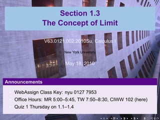
1. Section 1.3
The Concept of Limit
V63.0121.002.2010Su, Calculus I
New York University
May 18, 2010
Announcements
WebAssign Class Key: nyu 0127 7953
Office Hours: MR 5:00–5:45, TW 7:50–8:30, CIWW 102 (here)
Quiz 1 Thursday on 1.1–1.4
. . . . . .
2. Announcements
WebAssign Class Key: nyu
0127 7953
Office Hours: MR
5:00–5:45, TW 7:50–8:30,
CIWW 102 (here)
Quiz 1 Thursday on
1.1–1.4
. . . . . .
V63.0121.002.2010Su, Calculus I (NYU) Section 1.3 The Concept of Limit May 18, 2010 2 / 32
3. Objectives
Understand and state the
informal definition of a limit.
Observe limits on a graph.
Guess limits by algebraic
manipulation.
Guess limits by numerical
information.
. . . . . .
V63.0121.002.2010Su, Calculus I (NYU) Section 1.3 The Concept of Limit May 18, 2010 3 / 32
4. Last Time
Key concept: function
Properties of functions: domain and range
Kinds of functions: linear, polynomial, power, rational, algebraic,
transcendental.
. . . . . .
V63.0121.002.2010Su, Calculus I (NYU) Section 1.3 The Concept of Limit May 18, 2010 4 / 32
6. Zeno's Paradox
That which is in
locomotion must arrive
at the half-way stage
before it arrives at the
goal.
(Aristotle Physics VI:9, 239b10)
. . . . . .
V63.0121.002.2010Su, Calculus I (NYU) Section 1.3 The Concept of Limit May 18, 2010 5 / 32
7. Outline
Heuristics
Errors and tolerances
Examples
Pathologies
Precise Definition of a Limit
. . . . . .
V63.0121.002.2010Su, Calculus I (NYU) Section 1.3 The Concept of Limit May 18, 2010 6 / 32
8. Heuristic Definition of a Limit
Definition
We write
lim f(x) = L
x→a
and say
“the limit of f(x), as x approaches a, equals L”
if we can make the values of f(x) arbitrarily close to L (as close to L as
we like) by taking x to be sufficiently close to a (on either side of a) but
not equal to a.
. . . . . .
V63.0121.002.2010Su, Calculus I (NYU) Section 1.3 The Concept of Limit May 18, 2010 7 / 32
9. Outline
Heuristics
Errors and tolerances
Examples
Pathologies
Precise Definition of a Limit
. . . . . .
V63.0121.002.2010Su, Calculus I (NYU) Section 1.3 The Concept of Limit May 18, 2010 8 / 32
10. The error-tolerance game
A game between two players to decide if a limit lim f(x) exists.
x→a
Step 1 Player 1 proposes L to be the limit.
Step 2 Player 2 chooses an “error” level around L: the maximum
amount f(x) can be away from L.
Step 3 Player 1 looks for a “tolerance” level around a: the maximum
amount x can be from a while ensuring f(x) is within the given
error of L. The idea is that points x within the tolerance level of
a are taken by f to y-values within the error level of L, with the
possible exception of a itself.
If Player 1 can do this, he wins the round. If he cannot, he
loses the game: the limit cannot be L.
Step 4 Player 2 go back to Step 2 with a smaller error. Or, he can give
up and concede that the limit is L.
. . . . . .
V63.0121.002.2010Su, Calculus I (NYU) Section 1.3 The Concept of Limit May 18, 2010 9 / 32
11. The error-tolerance game
L
.
.
a
.
. . . . . .
V63.0121.002.2010Su, Calculus I (NYU) Section 1.3 The Concept of Limit May 18, 2010 10 / 32
12. The error-tolerance game
L
.
.
a
.
. . . . . .
V63.0121.002.2010Su, Calculus I (NYU) Section 1.3 The Concept of Limit May 18, 2010 10 / 32
13. The error-tolerance game
L
.
.
a
.
To be legit, the part of the graph inside the blue (vertical) strip
must also be inside the green (horizontal) strip.
. . . . . .
V63.0121.002.2010Su, Calculus I (NYU) Section 1.3 The Concept of Limit May 18, 2010 10 / 32
14. The error-tolerance game
T
. his tolerance is too big
L
.
.
a
.
To be legit, the part of the graph inside the blue (vertical) strip
must also be inside the green (horizontal) strip.
. . . . . .
V63.0121.002.2010Su, Calculus I (NYU) Section 1.3 The Concept of Limit May 18, 2010 10 / 32
15. The error-tolerance game
L
.
.
a
.
To be legit, the part of the graph inside the blue (vertical) strip
must also be inside the green (horizontal) strip.
. . . . . .
V63.0121.002.2010Su, Calculus I (NYU) Section 1.3 The Concept of Limit May 18, 2010 10 / 32
16. The error-tolerance game
S
. till too big
L
.
.
a
.
To be legit, the part of the graph inside the blue (vertical) strip
must also be inside the green (horizontal) strip.
. . . . . .
V63.0121.002.2010Su, Calculus I (NYU) Section 1.3 The Concept of Limit May 18, 2010 10 / 32
17. The error-tolerance game
L
.
.
a
.
To be legit, the part of the graph inside the blue (vertical) strip
must also be inside the green (horizontal) strip.
. . . . . .
V63.0121.002.2010Su, Calculus I (NYU) Section 1.3 The Concept of Limit May 18, 2010 10 / 32
18. The error-tolerance game
T
. his looks good
L
.
.
a
.
To be legit, the part of the graph inside the blue (vertical) strip
must also be inside the green (horizontal) strip.
. . . . . .
V63.0121.002.2010Su, Calculus I (NYU) Section 1.3 The Concept of Limit May 18, 2010 10 / 32
19. The error-tolerance game
S
. o does this
L
.
.
a
.
To be legit, the part of the graph inside the blue (vertical) strip
must also be inside the green (horizontal) strip.
. . . . . .
V63.0121.002.2010Su, Calculus I (NYU) Section 1.3 The Concept of Limit May 18, 2010 10 / 32
20. The error-tolerance game
L
.
.
a
.
To be legit, the part of the graph inside the blue (vertical) strip
must also be inside the green (horizontal) strip.
If Player 2 shrinks the error, Player 1 can still win.
. . . . . .
V63.0121.002.2010Su, Calculus I (NYU) Section 1.3 The Concept of Limit May 18, 2010 10 / 32
21. The error-tolerance game
L
.
.
a
.
To be legit, the part of the graph inside the blue (vertical) strip
must also be inside the green (horizontal) strip.
If Player 2 shrinks the error, Player 1 can still win.
. . . . . .
V63.0121.002.2010Su, Calculus I (NYU) Section 1.3 The Concept of Limit May 18, 2010 10 / 32
22. Outline
Heuristics
Errors and tolerances
Examples
Pathologies
Precise Definition of a Limit
. . . . . .
V63.0121.002.2010Su, Calculus I (NYU) Section 1.3 The Concept of Limit May 18, 2010 11 / 32
23. Playing the Error-Tolerance game with x2
Example
Find lim x2 if it exists.
x→0
. . . . . .
V63.0121.002.2010Su, Calculus I (NYU) Section 1.3 The Concept of Limit May 18, 2010 12 / 32
24. Playing the Error-Tolerance game with x2
Example
Find lim x2 if it exists.
x→0
Solution
Step 1 Player 1: I claim the limit is zero.
. . . . . .
V63.0121.002.2010Su, Calculus I (NYU) Section 1.3 The Concept of Limit May 18, 2010 12 / 32
25. Playing the Error-Tolerance game with x2
Example
Find lim x2 if it exists.
x→0
Solution
Step 1 Player 1: I claim the limit is zero.
Step 2 Player 2: I challenge you to make x2 within 0.01 of 0.
. . . . . .
V63.0121.002.2010Su, Calculus I (NYU) Section 1.3 The Concept of Limit May 18, 2010 12 / 32
26. Playing the Error-Tolerance game with x2
Example
Find lim x2 if it exists.
x→0
Solution
Step 1 Player 1: I claim the limit is zero.
Step 2 Player 2: I challenge you to make x2 within 0.01 of 0.
Step 3 Player 1: That’s easy. If −0.1 < x < 0.1, then 0 ≤ x2 < 0.01,
so a tolerance of 0.1 fits your error of 0.01.
. . . . . .
V63.0121.002.2010Su, Calculus I (NYU) Section 1.3 The Concept of Limit May 18, 2010 12 / 32
27. Playing the Error-Tolerance game with x2
Example
Find lim x2 if it exists.
x→0
Solution
Step 1 Player 1: I claim the limit is zero.
Step 2 Player 2: I challenge you to make x2 within 0.01 of 0.
Step 3 Player 1: That’s easy. If −0.1 < x < 0.1, then 0 ≤ x2 < 0.01,
so a tolerance of 0.1 fits your error of 0.01.
Step 4 Player 2: OK, smart guy. Can you make x2 within 0.0001 of 0?
. . . . . .
V63.0121.002.2010Su, Calculus I (NYU) Section 1.3 The Concept of Limit May 18, 2010 12 / 32
28. Playing the Error-Tolerance game with x2
Example
Find lim x2 if it exists.
x→0
Solution
Step 1 Player 1: I claim the limit is zero.
Step 2 Player 2: I challenge you to make x2 within 0.01 of 0.
Step 3 Player 1: That’s easy. If −0.1 < x < 0.1, then 0 ≤ x2 < 0.01,
so a tolerance of 0.1 fits your error of 0.01.
Step 4 Player 2: OK, smart guy. Can you make x2 within 0.0001 of 0?
Step 5 Player 1: Sure. If −0.01 < x < 0.01, then 0 ≤ x2 < 0.0001, so
a tolerance of 0.01 fits your error of 0.0001. …
. . . . . .
V63.0121.002.2010Su, Calculus I (NYU) Section 1.3 The Concept of Limit May 18, 2010 12 / 32
29. Playing the Error-Tolerance game with x2
Example
Find lim x2 if it exists.
x→0
Solution
Step 1 Player 1: I claim the limit is zero.
Step 2 Player 2: I challenge you to make x2 within 0.01 of 0.
Step 3 Player 1: That’s easy. If −0.1 < x < 0.1, then 0 ≤ x2 < 0.01,
so a tolerance of 0.1 fits your error of 0.01.
Step 4 Player 2: OK, smart guy. Can you make x2 within 0.0001 of 0?
Step 5 Player 1: Sure. If −0.01 < x < 0.01, then 0 ≤ x2 < 0.0001, so
a tolerance of 0.01 fits your error of 0.0001. …
Can you convince Player 2 that Player 1 can win every round?
. . . . . .
V63.0121.002.2010Su, Calculus I (NYU) Section 1.3 The Concept of Limit May 18, 2010 12 / 32
30. Playing the Error-Tolerance game with x2
Example
Find lim x2 if it exists.
x→0
Solution
Step 1 Player 1: I claim the limit is zero.
Step 2 Player 2: I challenge you to make x2 within 0.01 of 0.
Step 3 Player 1: That’s easy. If −0.1 < x < 0.1, then 0 ≤ x2 < 0.01,
so a tolerance of 0.1 fits your error of 0.01.
Step 4 Player 2: OK, smart guy. Can you make x2 within 0.0001 of 0?
Step 5 Player 1: Sure. If −0.01 < x < 0.01, then 0 ≤ x2 < 0.0001, so
a tolerance of 0.01 fits your error of 0.0001. …
Can you convince Player 2 that Player 1 can win every round? Yes, by
setting the tolerance equal to the square root of the error, Player 1 can
always win. Player 2 should give up and concede that the limit is 0. . . . . . .
V63.0121.002.2010Su, Calculus I (NYU) Section 1.3 The Concept of Limit May 18, 2010 12 / 32
31. Graphical version of the E-T game with x2
. .
y
. . .
x
.
.
. . . . . .
V63.0121.002.2010Su, Calculus I (NYU) Section 1.3 The Concept of Limit May 18, 2010 13 / 32
32. Graphical version of the E-T game with x2
. .
y
. . .
x
.
.
. . . . . .
V63.0121.002.2010Su, Calculus I (NYU) Section 1.3 The Concept of Limit May 18, 2010 13 / 32
33. Graphical version of the E-T game with x2
. .
y
. . .
x
.
.
. . . . . .
V63.0121.002.2010Su, Calculus I (NYU) Section 1.3 The Concept of Limit May 18, 2010 13 / 32
34. Graphical version of the E-T game with x2
. .
y
. . .
x
.
.
. . . . . .
V63.0121.002.2010Su, Calculus I (NYU) Section 1.3 The Concept of Limit May 18, 2010 13 / 32
35. Graphical version of the E-T game with x2
. .
y
. . .
x
.
.
. . . . . .
V63.0121.002.2010Su, Calculus I (NYU) Section 1.3 The Concept of Limit May 18, 2010 13 / 32
36. Graphical version of the E-T game with x2
. .
y
. . .
x
.
.
. . . . . .
V63.0121.002.2010Su, Calculus I (NYU) Section 1.3 The Concept of Limit May 18, 2010 13 / 32
37. Graphical version of the E-T game with x2
. .
y
. . .
x
.
.
. . . . . .
V63.0121.002.2010Su, Calculus I (NYU) Section 1.3 The Concept of Limit May 18, 2010 13 / 32
38. Graphical version of the E-T game with x2
. .
y
. . .
x
.
.
. . . . . .
V63.0121.002.2010Su, Calculus I (NYU) Section 1.3 The Concept of Limit May 18, 2010 13 / 32
39. Graphical version of the E-T game with x2
. .
y
. . .
x
.
.
No matter how small an error band Player 2 picks, Player 1 can
find a fitting tolerance band.
. . . . . .
V63.0121.002.2010Su, Calculus I (NYU) Section 1.3 The Concept of Limit May 18, 2010 13 / 32
40. Limit of a piecewise function
Example
|x|
Find lim if it exists.
x→0 x
. . . . . .
V63.0121.002.2010Su, Calculus I (NYU) Section 1.3 The Concept of Limit May 18, 2010 14 / 32
41. Limit of a piecewise function
Example
|x|
Find lim if it exists.
x→0 x
Solution
The function can also be written as
{
|x| 1 if x > 0;
=
x −1 if x < 0
What would be the limit?
. . . . . .
V63.0121.002.2010Su, Calculus I (NYU) Section 1.3 The Concept of Limit May 18, 2010 14 / 32
42. The E-T game with a piecewise function
y
.
.
. . .
1
. . ..
x
. 1.
−
.
.
. . . . . .
V63.0121.002.2010Su, Calculus I (NYU) Section 1.3 The Concept of Limit May 18, 2010 15 / 32
43. The E-T game with a piecewise function
y
.
.
. . .
1
I
. think the limit is 1
. . ..
x
. 1.
−
.
.
. . . . . .
V63.0121.002.2010Su, Calculus I (NYU) Section 1.3 The Concept of Limit May 18, 2010 15 / 32
44. The E-T game with a piecewise function
y
.
.
. . .
1
I
. think the limit is 1
. . ..
x
C
. an you fit an error of 0.5?
. 1.
−
.
.
. . . . . .
V63.0121.002.2010Su, Calculus I (NYU) Section 1.3 The Concept of Limit May 18, 2010 15 / 32
45. The E-T game with a piecewise function
y
.
.
. . .
1
H
. ow about this for a tolerance?
. . ..
x
. 1.
−
.
.
. . . . . .
V63.0121.002.2010Su, Calculus I (NYU) Section 1.3 The Concept of Limit May 18, 2010 15 / 32
46. The E-T game with a piecewise function
y
.
.
. . .
1
H
. ow about this for a tolerance?
. . ..
x
.
No. Part of
graph inside
. 1.
−
blue is not inside
green
.
.
. . . . . .
V63.0121.002.2010Su, Calculus I (NYU) Section 1.3 The Concept of Limit May 18, 2010 15 / 32
47. The E-T game with a piecewise function
y
.
.
. . .
1
O
. h, I guess the limit isn’t 1
. . ..
x
.
No. Part of
graph inside
. 1.
−
blue is not inside
green
.
.
. . . . . .
V63.0121.002.2010Su, Calculus I (NYU) Section 1.3 The Concept of Limit May 18, 2010 15 / 32
48. The E-T game with a piecewise function
y
.
.
. . .
1
. think the limit is −1
I
. . ..
x
. 1.
−
.
.
. . . . . .
V63.0121.002.2010Su, Calculus I (NYU) Section 1.3 The Concept of Limit May 18, 2010 15 / 32
49. The E-T game with a piecewise function
y
.
.
. . .
1
. think the limit is −1
I
. . ..
x
C
. an you fit an error of 0.5?
. 1.
−
.
.
. . . . . .
V63.0121.002.2010Su, Calculus I (NYU) Section 1.3 The Concept of Limit May 18, 2010 15 / 32
50. The E-T game with a piecewise function
y
.
.
. . .
1
H
. ow about this for a tolerance?
. . ..
x
C
. an you fit an error of 0.5?
. 1.
−
.
.
. . . . . .
V63.0121.002.2010Su, Calculus I (NYU) Section 1.3 The Concept of Limit May 18, 2010 15 / 32
51. The E-T game with a piecewise function
y
.
.
.
No. Part of
. graph inside
. .
1
blue is not inside
. ow about this for a tolerance? green
H
. . ..
x
. 1.
−
.
.
. . . . . .
V63.0121.002.2010Su, Calculus I (NYU) Section 1.3 The Concept of Limit May 18, 2010 15 / 32
52. The E-T game with a piecewise function
y
.
.
.
No. Part of
. graph inside
. .
1
blue is not inside
. h, I guess the limit isn’t −1
O green
. . ..
x
. 1.
−
.
.
. . . . . .
V63.0121.002.2010Su, Calculus I (NYU) Section 1.3 The Concept of Limit May 18, 2010 15 / 32
53. The E-T game with a piecewise function
y
.
.
. . .
1
I
. think the limit is 0
. . ..
x
. 1.
−
.
.
. . . . . .
V63.0121.002.2010Su, Calculus I (NYU) Section 1.3 The Concept of Limit May 18, 2010 15 / 32
54. The E-T game with a piecewise function
y
.
.
. . .
1
I
. think the limit is 0
. . ..
x
C
. an you fit an error of 0.5?
. 1.
−
.
.
. . . . . .
V63.0121.002.2010Su, Calculus I (NYU) Section 1.3 The Concept of Limit May 18, 2010 15 / 32
55. The E-T game with a piecewise function
y
.
.
. . .
1
H
. ow about this for a tolerance?
. . ..
x
C
. an you fit an error of 0.5?
. 1.
−
.
.
. . . . . .
V63.0121.002.2010Su, Calculus I (NYU) Section 1.3 The Concept of Limit May 18, 2010 15 / 32
56. The E-T game with a piecewise function
y
.
.
. . .
1
H
. ow about this for a tolerance?
. . ..
x
.
No. None of
. 1.
−
graph inside blue
is inside green
.
.
. . . . . .
V63.0121.002.2010Su, Calculus I (NYU) Section 1.3 The Concept of Limit May 18, 2010 15 / 32
57. The E-T game with a piecewise function
y
.
.
. . .
1
.
. Oh, I guess the . ..
x
limit isn’t 0
.
No. None of
. 1.
−
graph inside blue
is inside green
.
.
. . . . . .
V63.0121.002.2010Su, Calculus I (NYU) Section 1.3 The Concept of Limit May 18, 2010 15 / 32
58. The E-T game with a piecewise function
y
.
.
. . .
1
.
I give up! I
. guess there’s . ..
x
no limit!
. 1.
−
.
.
. . . . . .
V63.0121.002.2010Su, Calculus I (NYU) Section 1.3 The Concept of Limit May 18, 2010 15 / 32
59. One-sided limits
Definition
We write
lim f(x) = L
x→a+
and say
“the limit of f(x), as x approaches a from the right, equals L”
if we can make the values of f(x) arbitrarily close to L (as close to L as
we like) by taking x to be sufficiently close to a and greater than a.
. . . . . .
V63.0121.002.2010Su, Calculus I (NYU) Section 1.3 The Concept of Limit May 18, 2010 16 / 32
60. One-sided limits
Definition
We write
lim f(x) = L
x→a−
and say
“the limit of f(x), as x approaches a from the left, equals L”
if we can make the values of f(x) arbitrarily close to L (as close to L as
we like) by taking x to be sufficiently close to a and less than a.
. . . . . .
V63.0121.002.2010Su, Calculus I (NYU) Section 1.3 The Concept of Limit May 18, 2010 16 / 32
61. The error-tolerance game on the right
y
.
. .
1
. x
.
. 1.
−
. . . . . .
V63.0121.002.2010Su, Calculus I (NYU) Section 1.3 The Concept of Limit May 18, 2010 17 / 32
62. The error-tolerance game on the right
y
.
. .
1
. x
.
. 1.
−
. . . . . .
V63.0121.002.2010Su, Calculus I (NYU) Section 1.3 The Concept of Limit May 18, 2010 17 / 32
63. The error-tolerance game on the right
y
.
. .
1
. x
.
. 1.
−
. . . . . .
V63.0121.002.2010Su, Calculus I (NYU) Section 1.3 The Concept of Limit May 18, 2010 17 / 32
64. The error-tolerance game on the right
y
.
. .
1
. x
.
. 1.
−
. . . . . .
V63.0121.002.2010Su, Calculus I (NYU) Section 1.3 The Concept of Limit May 18, 2010 17 / 32
65. The error-tolerance game on the right
y
.
. .
1
. x
.
.
All of graph in-
. 1.
− side blue is in-
side green
. . . . . .
V63.0121.002.2010Su, Calculus I (NYU) Section 1.3 The Concept of Limit May 18, 2010 17 / 32
66. The error-tolerance game on the right
y
.
. .
1
. x
.
. 1.
−
. . . . . .
V63.0121.002.2010Su, Calculus I (NYU) Section 1.3 The Concept of Limit May 18, 2010 17 / 32
67. The error-tolerance game on the right
y
.
. .
1
. x
.
. 1.
−
. . . . . .
V63.0121.002.2010Su, Calculus I (NYU) Section 1.3 The Concept of Limit May 18, 2010 17 / 32
68. The error-tolerance game on the right
y
.
. .
1
. x
.
. 1.
−
. . . . . .
V63.0121.002.2010Su, Calculus I (NYU) Section 1.3 The Concept of Limit May 18, 2010 17 / 32
69. The error-tolerance game on the right
y
.
.
All of graph in- . .
1
side blue is in-
side green
. x
.
. 1.
−
. . . . . .
V63.0121.002.2010Su, Calculus I (NYU) Section 1.3 The Concept of Limit May 18, 2010 17 / 32
70. The error-tolerance game on the right
y
.
.
All of graph in- . .
1
side blue is in-
side green
. x
.
. 1.
−
So lim+ f(x) = 1 and lim f(x) = −1
x→0 x→0−
. . . . . .
V63.0121.002.2010Su, Calculus I (NYU) Section 1.3 The Concept of Limit May 18, 2010 17 / 32
71. Limit of a piecewise function
Example
|x|
Find lim if it exists.
x→0 x
Solution
The function can also be written as
{
|x| 1 if x > 0;
=
x −1 if x < 0
What would be the limit?
The error-tolerance game fails, but
lim f(x) = 1 lim f(x) = −1
x→0+ x→0−
. . . . . .
V63.0121.002.2010Su, Calculus I (NYU) Section 1.3 The Concept of Limit May 18, 2010 18 / 32
72. Another Example
Example
1
Find lim+ if it exists.
x→0 x
. . . . . .
V63.0121.002.2010Su, Calculus I (NYU) Section 1.3 The Concept of Limit May 18, 2010 19 / 32
73. The error-tolerance game with lim (1/x)
x→0
y
.
.?.
L
. x
.
0
.
. . . . . .
V63.0121.002.2010Su, Calculus I (NYU) Section 1.3 The Concept of Limit May 18, 2010 20 / 32
74. The error-tolerance game with lim (1/x)
x→0
y
.
.?.
L
. x
.
0
.
. . . . . .
V63.0121.002.2010Su, Calculus I (NYU) Section 1.3 The Concept of Limit May 18, 2010 20 / 32
75. The error-tolerance game with lim (1/x)
x→0
y
.
.?.
L
. x
.
0
.
. . . . . .
V63.0121.002.2010Su, Calculus I (NYU) Section 1.3 The Concept of Limit May 18, 2010 20 / 32
76. The error-tolerance game with lim (1/x)
x→0
y
.
.
The graph escapes
the green, so no good
.?.
L
. x
.
0
.
. . . . . .
V63.0121.002.2010Su, Calculus I (NYU) Section 1.3 The Concept of Limit May 18, 2010 20 / 32
77. The error-tolerance game with lim (1/x)
x→0
y
.
.?.
L
. x
.
0
.
. . . . . .
V63.0121.002.2010Su, Calculus I (NYU) Section 1.3 The Concept of Limit May 18, 2010 20 / 32
78. The error-tolerance game with lim (1/x)
x→0
y
.
E
. ven worse!
.?.
L
. x
.
0
.
. . . . . .
V63.0121.002.2010Su, Calculus I (NYU) Section 1.3 The Concept of Limit May 18, 2010 20 / 32
79. The error-tolerance game with lim (1/x)
x→0
y
.
.
The limit does not ex-
ist because the func-
tion is unbounded near
0
.?.
L
. x
.
0
.
. . . . . .
V63.0121.002.2010Su, Calculus I (NYU) Section 1.3 The Concept of Limit May 18, 2010 20 / 32
80. Another (Bad) Example: Unboundedness
Example
1
Find lim+ if it exists.
x→0 x
Solution
The limit does not exist because the function is unbounded near 0.
Later we will talk about the statement that
1
lim+ = +∞
x→0 x
. . . . . .
V63.0121.002.2010Su, Calculus I (NYU) Section 1.3 The Concept of Limit May 18, 2010 21 / 32
81. Weird, wild stuff
Example
(π )
Find lim sin if it exists.
x→0 x
. . . . . .
V63.0121.002.2010Su, Calculus I (NYU) Section 1.3 The Concept of Limit May 18, 2010 22 / 32
83. Weird, wild stuff
Example
(π )
Find lim sin if it exists.
x→0 x
. . . . . .
V63.0121.002.2010Su, Calculus I (NYU) Section 1.3 The Concept of Limit May 18, 2010 24 / 32
84. Weird, wild stuff
Example
(π )
Find lim sin if it exists.
x→0 x
f(x) = 0 when x =
f(x) = 1 when x =
f(x) = −1 when x =
. . . . . .
V63.0121.002.2010Su, Calculus I (NYU) Section 1.3 The Concept of Limit May 18, 2010 24 / 32
85. Weird, wild stuff
Example
(π )
Find lim sin if it exists.
x→0 x
1
f(x) = 0 when x = for any integer k
k
f(x) = 1 when x =
f(x) = −1 when x =
. . . . . .
V63.0121.002.2010Su, Calculus I (NYU) Section 1.3 The Concept of Limit May 18, 2010 24 / 32
86. Weird, wild stuff
Example
(π )
Find lim sin if it exists.
x→0 x
1
f(x) = 0 when x = for any integer k
k
2
f(x) = 1 when x = for any integer k
4k + 1
f(x) = −1 when x =
. . . . . .
V63.0121.002.2010Su, Calculus I (NYU) Section 1.3 The Concept of Limit May 18, 2010 24 / 32
87. Weird, wild stuff
Example
(π )
Find lim sin if it exists.
x→0 x
1
f(x) = 0 when x = for any integer k
k
2
f(x) = 1 when x = for any integer k
4k + 1
2
f(x) = −1 when x = for any integer k
4k − 1
. . . . . .
V63.0121.002.2010Su, Calculus I (NYU) Section 1.3 The Concept of Limit May 18, 2010 24 / 32
88. Weird, wild stuff continued
Here is a graph of the function:
y
.
. .
1
. x
.
. 1.
−
There are infinitely many points arbitrarily close to zero where f(x) is 0,
or 1, or −1. So the limit cannot exist.
. . . . . .
V63.0121.002.2010Su, Calculus I (NYU) Section 1.3 The Concept of Limit May 18, 2010 25 / 32
89. Outline
Heuristics
Errors and tolerances
Examples
Pathologies
Precise Definition of a Limit
. . . . . .
V63.0121.002.2010Su, Calculus I (NYU) Section 1.3 The Concept of Limit May 18, 2010 26 / 32
90. What could go wrong?
Summary of Limit Pathologies
How could a function fail to have a limit? Some possibilities:
left- and right- hand limits exist but are not equal
The function is unbounded near a
Oscillation with increasingly high frequency near a
. . . . . .
V63.0121.002.2010Su, Calculus I (NYU) Section 1.3 The Concept of Limit May 18, 2010 27 / 32
91. Meet the Mathematician: Augustin Louis Cauchy
French, 1789–1857
Royalist and Catholic
made contributions in
geometry, calculus,
complex analysis, number
theory
created the definition of
limit we use today but
didn’t understand it
. . . . . .
V63.0121.002.2010Su, Calculus I (NYU) Section 1.3 The Concept of Limit May 18, 2010 28 / 32
92. Outline
Heuristics
Errors and tolerances
Examples
Pathologies
Precise Definition of a Limit
. . . . . .
V63.0121.002.2010Su, Calculus I (NYU) Section 1.3 The Concept of Limit May 18, 2010 29 / 32
93. Precise Definition of a Limit
No, this is not going to be on the test
Let f be a function defined on an some open interval that contains the
number a, except possibly at a itself. Then we say that the limit of f(x)
as x approaches a is L, and we write
lim f(x) = L,
x→a
if for every ε > 0 there is a corresponding δ > 0 such that
if 0 < |x − a| < δ, then |f(x) − L| < ε.
. . . . . .
V63.0121.002.2010Su, Calculus I (NYU) Section 1.3 The Concept of Limit May 18, 2010 30 / 32
94. The error-tolerance game = ε, δ
L
.
.
a
.
. . . . . .
V63.0121.002.2010Su, Calculus I (NYU) Section 1.3 The Concept of Limit May 18, 2010 31 / 32
95. The error-tolerance game = ε, δ
L
. +ε
L
.
. −ε
L
.
a
.
. . . . . .
V63.0121.002.2010Su, Calculus I (NYU) Section 1.3 The Concept of Limit May 18, 2010 31 / 32
96. The error-tolerance game = ε, δ
L
. +ε
L
.
. −ε
L
.
. − δ. . + δ
a aa
. . . . . .
V63.0121.002.2010Su, Calculus I (NYU) Section 1.3 The Concept of Limit May 18, 2010 31 / 32
97. The error-tolerance game = ε, δ
T
. his δ is too big
L
. +ε
L
.
. −ε
L
.
. − δ. . + δ
a aa
. . . . . .
V63.0121.002.2010Su, Calculus I (NYU) Section 1.3 The Concept of Limit May 18, 2010 31 / 32
98. The error-tolerance game = ε, δ
L
. +ε
L
.
. −ε
L
.
. −. δ δ
a . a+
a
. . . . . .
V63.0121.002.2010Su, Calculus I (NYU) Section 1.3 The Concept of Limit May 18, 2010 31 / 32
99. The error-tolerance game = ε, δ
T
. his δ looks good
L
. +ε
L
.
. −ε
L
.
. −. δ δ
a . a+
a
. . . . . .
V63.0121.002.2010Su, Calculus I (NYU) Section 1.3 The Concept of Limit May 18, 2010 31 / 32
100. The error-tolerance game = ε, δ
S
. o does this δ
L
. +ε
L
.
. −ε
L
.
. .− δ δ
aa .+
a
. . . . . .
V63.0121.002.2010Su, Calculus I (NYU) Section 1.3 The Concept of Limit May 18, 2010 31 / 32
101. Summary
y
.
Fundamental Concept: . .
1
limit
Error-Tolerance game . x
.
gives a methods of arguing
limits do or do not exist
Limit FAIL: jumps,
. 1.
−
unboundedness, sin(π/x)
FAIL
.
. . . . . .
V63.0121.002.2010Su, Calculus I (NYU) Section 1.3 The Concept of Limit May 18, 2010 32 / 32