Downloaded 174 times


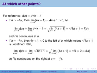
![Why a sum of continuous functions is continuous
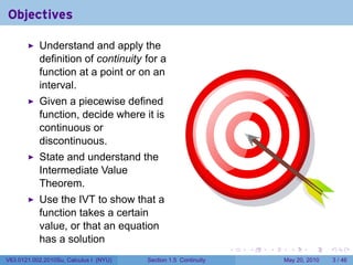
We want to show that
lim (f + g)(x) = (f + g)(a).
x→a
We just follow our nose:
lim (f + g)(x) = lim [f(x) + g(x)] (def of f + g)
x→a x→a
= lim f(x) + lim g(x) (if these limits exist)
x→a x→a
= f(a) + g(a) (they do; f and g are cts.)
= (f + g)(a) (def of f + g again)
. . . . . .
V63.0121.002.2010Su, Calculus I (NYU) Section 1.5 Continuity May 20, 2010 16 / 46](https://image.slidesharecdn.com/lesson04-continuityslides-100520064223-phpapp02/85/Lesson-4-Continuity-23-320.jpg)
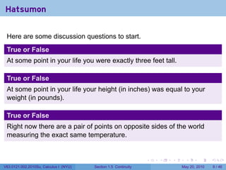
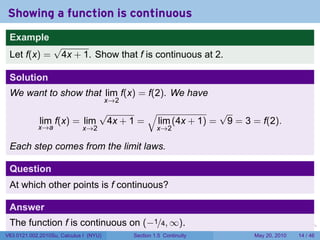
![Continuity FAIL: The limit does not exist
.
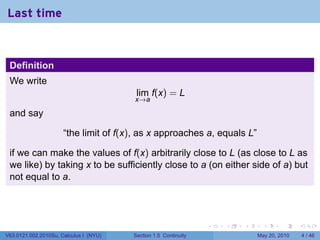
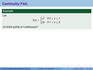
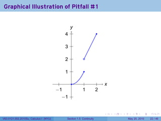
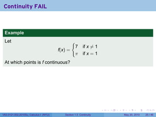
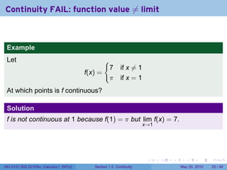
Example
Let {
x2 if 0 ≤ x ≤ 1
f(x) =
2x if 1 < x ≤ 2
At which points is f continuous?
Solution
At any point a in [0, 2] besides 1, lim f(x) = f(a) because f is represented by a
x→a
polynomial near a, and polynomials have the direct substitution property.
However,
lim f(x) = lim x2 = 12 = 1
x→1− x→1−
lim f(x) = lim+ 2x = 2(1) = 2
x→1+ x→1
So f has no limit at 1. Therefore f is not continuous at 1.
.
. . . . . .
V63.0121.002.2010Su, Calculus I (NYU) Section 1.5 Continuity May 20, 2010 21 / 46](https://image.slidesharecdn.com/lesson04-continuityslides-100520064223-phpapp02/85/Lesson-4-Continuity-41-320.jpg)
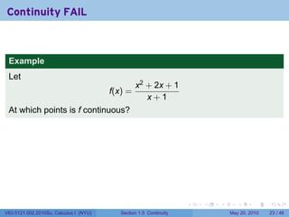
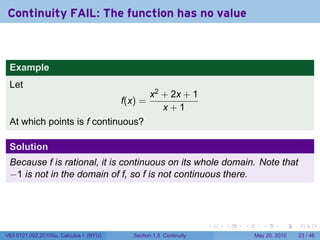
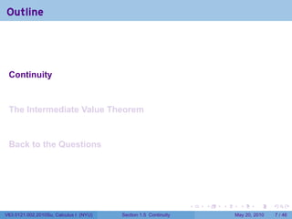
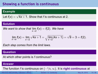
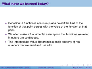
![The greatest integer function
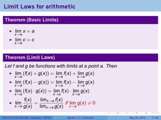
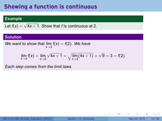
[[x]] is the greatest integer ≤ x.
y
.
. .
3
x [[x]] y
. = [[x]]
0 0 . .
2 . .
1 1
1.5 1 . .
1 . .
1.9 1
2.1 2 . . . . . . x
.
−0.5 −1 −
. 2 −
. 1 1
. 2
. 3
.
−0.9 −1 .. 1 .
−
−1.1 −2
. .. 2 .
−
. . . . . .
V63.0121.002.2010Su, Calculus I (NYU) Section 1.5 Continuity May 20, 2010 30 / 46](https://image.slidesharecdn.com/lesson04-continuityslides-100520064223-phpapp02/85/Lesson-4-Continuity-57-320.jpg)
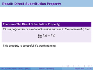
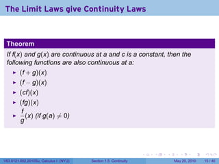
![The greatest integer function
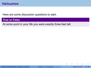
[[x]] is the greatest integer ≤ x.
y
.
. .
3
x [[x]] y
. = [[x]]
0 0 . .
2 . .
1 1
1.5 1 . .
1 . .
1.9 1
2.1 2 . . . . . . x
.
−0.5 −1 −
. 2 −
. 1 1
. 2
. 3
.
−0.9 −1 .. 1 .
−
−1.1 −2
. .. 2 .
−
This function has a jump discontinuity at each integer.
. . . . . .
V63.0121.002.2010Su, Calculus I (NYU) Section 1.5 Continuity May 20, 2010 30 / 46](https://image.slidesharecdn.com/lesson04-continuityslides-100520064223-phpapp02/85/Lesson-4-Continuity-58-320.jpg)
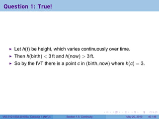
![A Big Time Theorem
Theorem (The Intermediate Value Theorem)
Suppose that f is continuous on the closed interval [a, b] and let N be
any number between f(a) and f(b), where f(a) ̸= f(b). Then there
exists a number c in (a, b) such that f(c) = N.
. . . . . .
V63.0121.002.2010Su, Calculus I (NYU) Section 1.5 Continuity May 20, 2010 32 / 46](https://image.slidesharecdn.com/lesson04-continuityslides-100520064223-phpapp02/85/Lesson-4-Continuity-60-320.jpg)

![Illustrating the IVT
Suppose that f is continuous on the closed interval [a, b]
f
.(x)
.
.
. x
.
. . . . . .
V63.0121.002.2010Su, Calculus I (NYU) Section 1.5 Continuity May 20, 2010 33 / 46](https://image.slidesharecdn.com/lesson04-continuityslides-100520064223-phpapp02/85/Lesson-4-Continuity-62-320.jpg)
![Illustrating the IVT
Suppose that f is continuous on the closed interval [a, b]
f
.(x)
f
.(b) .
f
.(a) .
. x
.
a
. b
.
. . . . . .
V63.0121.002.2010Su, Calculus I (NYU) Section 1.5 Continuity May 20, 2010 33 / 46](https://image.slidesharecdn.com/lesson04-continuityslides-100520064223-phpapp02/85/Lesson-4-Continuity-63-320.jpg)
![Illustrating the IVT
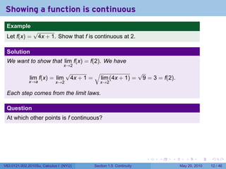
Suppose that f is continuous on the closed interval [a, b] and let N be
any number between f(a) and f(b), where f(a) ̸= f(b).
f
.(x)
f
.(b) .
N
.
f
.(a) .
. x
.
a
. b
.
. . . . . .
V63.0121.002.2010Su, Calculus I (NYU) Section 1.5 Continuity May 20, 2010 33 / 46](https://image.slidesharecdn.com/lesson04-continuityslides-100520064223-phpapp02/85/Lesson-4-Continuity-64-320.jpg)
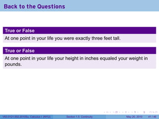
![Illustrating the IVT
Suppose that f is continuous on the closed interval [a, b] and let N be
any number between f(a) and f(b), where f(a) ̸= f(b). Then there
exists a number c in (a, b) such that f(c) = N.
f
.(x)
f
.(b) .
N
. .
f
.(a) .
. x
.
a
. c
. b
.
. . . . . .
V63.0121.002.2010Su, Calculus I (NYU) Section 1.5 Continuity May 20, 2010 33 / 46](https://image.slidesharecdn.com/lesson04-continuityslides-100520064223-phpapp02/85/Lesson-4-Continuity-65-320.jpg)
![Illustrating the IVT
Suppose that f is continuous on the closed interval [a, b] and let N be
any number between f(a) and f(b), where f(a) ̸= f(b). Then there
exists a number c in (a, b) such that f(c) = N.
f
.(x)
f
.(b) .
N
.
f
.(a) .
. x
.
a
. b
.
. . . . . .
V63.0121.002.2010Su, Calculus I (NYU) Section 1.5 Continuity May 20, 2010 33 / 46](https://image.slidesharecdn.com/lesson04-continuityslides-100520064223-phpapp02/85/Lesson-4-Continuity-66-320.jpg)
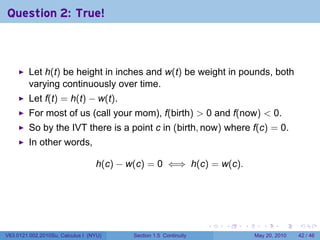
![Illustrating the IVT
Suppose that f is continuous on the closed interval [a, b] and let N be
any number between f(a) and f(b), where f(a) ̸= f(b). Then there
exists a number c in (a, b) such that f(c) = N.
f
.(x)
f
.(b) .
N
. . . .
f
.(a) .
. x
.
ac
. .1 c
.2 c b
.3 .
. . . . . .
V63.0121.002.2010Su, Calculus I (NYU) Section 1.5 Continuity May 20, 2010 33 / 46](https://image.slidesharecdn.com/lesson04-continuityslides-100520064223-phpapp02/85/Lesson-4-Continuity-67-320.jpg)
![Using the IVT
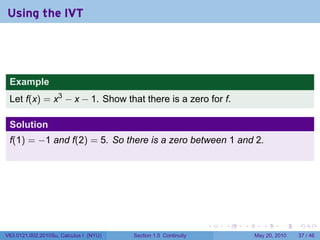
Example
Suppose we are unaware of the square root function and that it’s
continuous. Prove that the square root of two exists.
Proof.
Let f(x) = x2 , a continuous function on [1, 2].
. . . . . .
V63.0121.002.2010Su, Calculus I (NYU) Section 1.5 Continuity May 20, 2010 35 / 46](https://image.slidesharecdn.com/lesson04-continuityslides-100520064223-phpapp02/85/Lesson-4-Continuity-70-320.jpg)
![Using the IVT
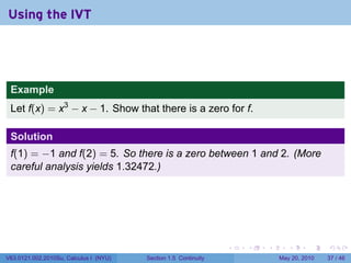
Example
Suppose we are unaware of the square root function and that it’s
continuous. Prove that the square root of two exists.
Proof.
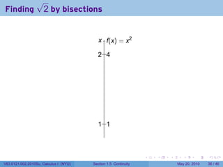
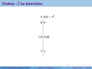
Let f(x) = x2 , a continuous function on [1, 2]. Note f(1) = 1 and
f(2) = 4. Since 2 is between 1 and 4, there exists a point c in (1, 2)
such that
f(c) = c2 = 2.
. . . . . .
V63.0121.002.2010Su, Calculus I (NYU) Section 1.5 Continuity May 20, 2010 35 / 46](https://image.slidesharecdn.com/lesson04-continuityslides-100520064223-phpapp02/85/Lesson-4-Continuity-71-320.jpg)
![Using the IVT
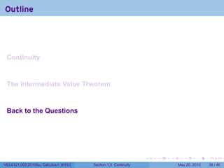
Example
Suppose we are unaware of the square root function and that it’s
continuous. Prove that the square root of two exists.
Proof.
Let f(x) = x2 , a continuous function on [1, 2]. Note f(1) = 1 and
f(2) = 4. Since 2 is between 1 and 4, there exists a point c in (1, 2)
such that
f(c) = c2 = 2.
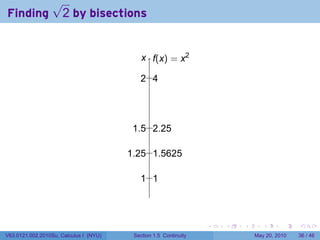
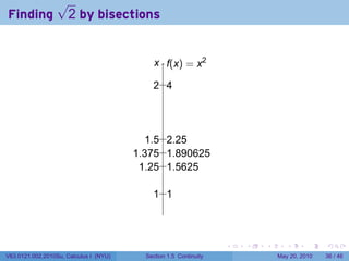
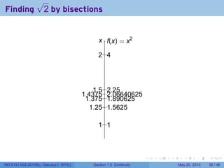
In fact, we can “narrow in” on the square root of 2 by the method of
bisections.
. . . . . .
V63.0121.002.2010Su, Calculus I (NYU) Section 1.5 Continuity May 20, 2010 35 / 46](https://image.slidesharecdn.com/lesson04-continuityslides-100520064223-phpapp02/85/Lesson-4-Continuity-72-320.jpg)


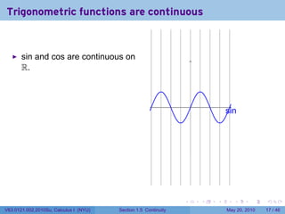
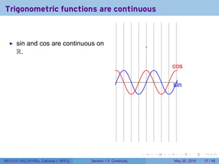
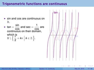
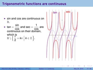
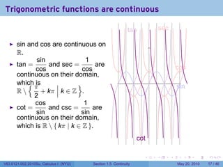
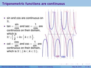
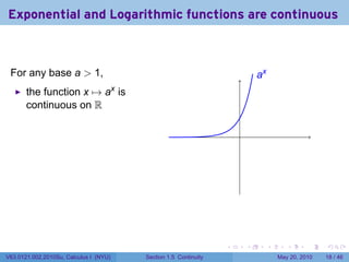
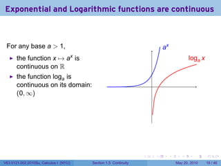
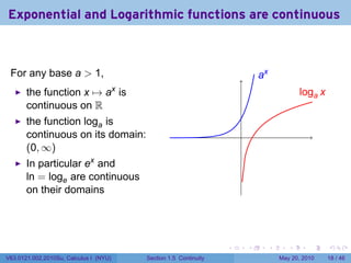
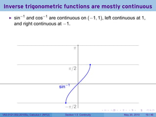
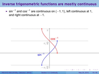
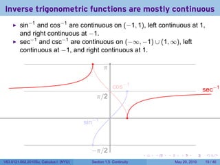
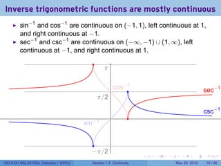
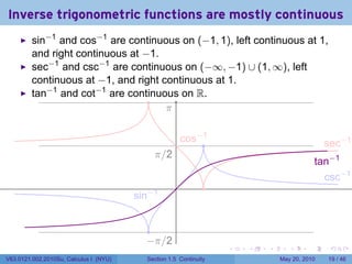
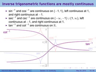
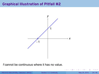
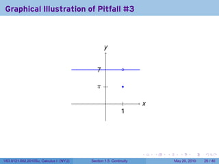
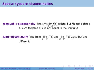
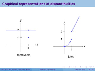
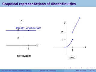
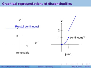
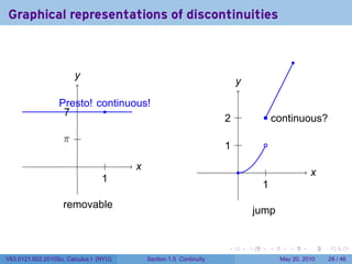
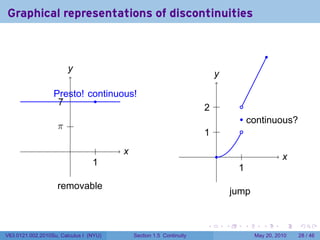
This document contains lecture notes from a Calculus I class at New York University. It discusses the definition of continuity for functions, examples of continuous and discontinuous functions, and properties of continuous functions like sums, products, and compositions of continuous functions being continuous. It also addresses trigonometric functions like sin, cos, tan, and sec being continuous on their domains.


![Limits and continuity[1]](https://cdn.slidesharecdn.com/ss_thumbnails/limitsandcontinuity1-110816105053-phpapp01-thumbnail.jpg?width=640&height=640&fit=bounds)


