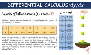
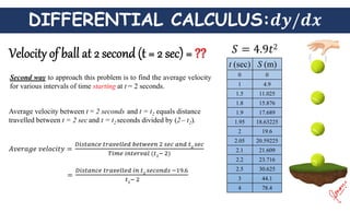
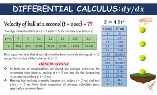
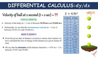
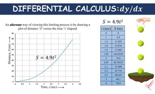
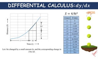
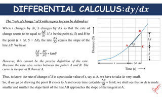
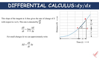
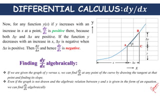
Introduction to differential calculus. This slide deals with the concept of differential calculus. An explanation is given that how derivative of a function can be calculated graphically and algebraically

2. DIFFERENTIAL CALCULUS:
One way to approach this problem is to find the average velocity for
various intervals of time ending at t = 2 seconds.
Average velocity between t = t1 and t = t2 equals distance travelled
between t = t1 and t = t2 seconds divided by (t2– t1).
Hence the average velocity in the first two seconds:
t (sec) S (m)
0 0
1 4.9
1.5 11.025
1.8 15.876
1.9 17.689
1.95 18.63225
2 19.6
2.05 20.59225
2.1 21.609
2.2 23.716
2.5 30.625
3 44.1
4 78.4

3. DIFFERENTIAL CALCULUS:
Similarly we can compute the average velocities between t = t1 and t = 2
for various t1 as follows:
t = t1 0 1 1.5 1.8 1.9 1.95 1.99
v 9.8 14.7 17.15 18.62 19.11 19.355 19.551
From the above table, it can be observed that the average velocity is
gradually increasing. As we make the time intervals ending at t = 2
smaller, we see that we get a better idea of the velocity at t = 2. Hoping
that nothing really dramatic happens between 1.99 seconds and 2
seconds, we conclude that the average velocity at t = 2 seconds is just
above 19.551m/s.
t (sec) S (m)
0 0
1 4.9
1.5 11.025
1.8 15.876
1.9 17.689
1.95 18.63225
2 19.6
2.05 20.59225
2.1 21.609
2.2 23.716
2.5 30.625
3 44.1
4 78.4

4. DIFFERENTIAL CALCULUS:
Second way to approach this problem is to find the average velocity
for various intervals of time starting at t = 2 seconds.
Average velocity between t = 2 seconds and t = t2 equals distance
travelled between t = 2 sec and t = t2seconds divided by (2– t2).
t (sec) S (m)
0 0
1 4.9
1.5 11.025
1.8 15.876
1.9 17.689
1.95 18.63225
2 19.6
2.05 20.59225
2.1 21.609
2.2 23.716
2.5 30.625
3 44.1
4 78.4

5. DIFFERENTIAL CALCULUS:
Average velocities between t = 2 and t = t2 for various t2 as follows:
t = t2 4 3 2.5 2.2 2.1 2.05 2.01
v 29.4 24.5 22.05 20.58 20.09 19.854 19.649
Here again we note that if we take smaller time intervals starting at t = 2,
we get better idea of the velocity at t = 2.
 In both set of computations we found the average velocities for
increasing time interval ending at t = 2 sec and for the decreasing
time interval ending at t = 2 sec.
 Hoping that nothing dramatic happen just before t = 2 sec and just
after t = 2 sec both these sequences of average velocities must
approach a common limit.
OBSERVATIONS:
t (sec) S (m)
0 0
1 4.9
1.5 11.025
1.8 15.876
1.9 17.689
1.95 18.63225
2 19.6
2.05 20.59225
2.1 21.609
2.2 23.716
2.5 30.625
3 44.1
4 78.4

6. DIFFERENTIAL CALCULUS:
 Velocity of the body at t = 2 sec is between 19.551m/s and 19.649 m/s.
 Technically, we say that the instantaneous velocity at t = 2 sec is
between 19.551 m/s and 19.649 m/s.
COCLUSIONS:
DISCUSSION:
 From the given data of distance covered at various time instants we
have estimated the rate of change of the distance at a given instant of
time.
 We say that the derivative of the distance function s = 4.9t2 at t = 2 is
between 19.551 and 19.649.
t (sec) S (m)
0 0
1 4.9
1.5 11.025
1.8 15.876
1.9 17.689
1.95 18.63225
2 19.6
2.05 20.59225
2.1 21.609
2.2 23.716
2.5 30.625
3 44.1
4 78.4

7. DIFFERENTIAL CALCULUS:
0
10
20
30
40
50
60
70
80
90
0 0.5 1 1.5 2 2.5 3 3.5 4 4.5
Time, t (sec)
Distance,
S
(m)
An alternate way of viewing this limiting process is by drawing a
plot of distance ‘S’ versus the time ‘t’ elapsed t (sec) S (m)
0 0
1 4.9
1.5 11.025
1.8 15.876
1.9 17.689
1.95 18.63225
2 19.6
2.05 20.59225
2.1 21.609
2.2 23.716
2.5 30.625
3 44.1
4 78.4

8. DIFFERENTIAL CALCULUS:
Time (t)
Distance
(S)
t Δt
S
ΔS
Let t be changed by a small amount Δt, and the corresponding change in
S be ΔS.
t (sec) S (m)
0 0
1 4.9
1.5 11.025
1.8 15.876
1.9 17.689
1.95 18.63225
2 19.6
2.05 20.59225
2.1 21.609
2.2 23.716
2.5 30.625
3 44.1
4 78.4

9. DIFFERENTIAL CALCULUS:
When t changes by Δt, S changes by ΔS so that the rate of
change seems to be equal to
ΔS
Δt
. If A be the point (t, S) and B be
the point (t + Δt, S + ΔS), the rate
ΔS
Δt
equals the slope of the
line AB. We have
Time (t)
Distance
(S)
t Δt
S
ΔS
θ
A
B
C
ΔS
Δt
=
BC
AC
=
However, this cannot be the precise definition of the rate.
Because the rate also varies between the points A and B. The
curve is steeper at B than at A.
Thus, to know the rate of change of S at a particular value of t, say at A, we have to take Δt very small.
So, if we go on drawing the point B closer to A and every time calculate
ΔS
Δt
= , we shall see that as Δt is made
smaller and smaller the slope of the line AB approaches the slope of the tangent at A.
The “rate of change” of S with respect to t can be defined as:

10. DIFFERENTIAL CALCULUS:
This slope of the tangent at A thus gives the rate of change of S
with respect to t at A. This rate is denoted by
dS
dt
Time (t)
Distance
(S)
t Δt
S
ΔS
θ
A
B
C
t
S
dt
dS
t 



 0
lim
For small changes Δt we can approximately write
t
dt
dS
S 



11. DIFFERENTIAL CALCULUS:
x
y
x Δx
y
Δy
θ
A
B
C
Now, for any function y(x) if y increases with an
increase in x at a point,
dy
d
is positive there, because
both Δy and Δx are positive. If the function y
decreases with an increase in x, Δy is negative when
Δx is positive. Then
y
and hence
dy
d
is negative.
 If we are given the graph of y versus x, we can find
dy
d
at any point of the curve by drawing the tangent at that
point and finding its slope.
 Even if the graph is not drawn and the algebraic relation between y and x is given in the form of an equation,
we can find
dy
d
algebraically
Finding
dy
d
algebraically:

12. DIFFERENTIAL CALCULUS:
L ΔL
L
ΔL
A
ΔA
2
L
A
, 
uare
Area of sq
2
ΔL)
L
(
ΔA
A 


L
ΔL
2
ΔL)
(
L
ΔA
A 2
2






L
ΔL
2
ΔL)
(
ΔA 2




L
2
ΔL
ΔL
ΔA



?
L
A

d
d
Now if ΔL is made smaller and smaller i.e. ΔL → 0, 2L + ΔL
will approach 2L.
L
2
ΔL
ΔA
lim
L
A
,
0
ΔL



d
d
Thus

13. DIFFERENTIAL CALCULUS:
2
A
, r
rcle
Area of ci 

2
)
Δ
(
ΔA
A r
r 

 
]
Δ
2
)
Δ
(
[
ΔA
A 2
2
r
r
r
r 




 
r
r
r 


 Δ
2
)
Δ
(
ΔA 2


r
r
r

 2
Δ
Δ
ΔA



?
A

dr
d
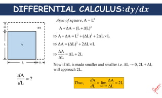
Now if Δr is made smaller and smaller i.e. Δr → 0, 2πr + πΔr
will approach 2πr.
r
r
dr
d
Thus
r

2
Δ
ΔA
lim
A
,
0
Δ



Δr
r
A
ΔA

14. for some common functions
1
)
( 
 n
n
nx
x
dx
d

15. for some common functions
x
x
dx
d
cos
)
(sin 

16. for some common functions
x
x
dx
d
sin
)
(cos 


17. for some common functions
x
x
dx
d 2
sec
)
(tan 

18. for some common functions
x
x
dx
d 2
cosec
)
(cot 


19. for some common functions
x
x
x
dx
d
tan
sec
)
(sec 


20. for some common functions
x
x
x
dx
d
cot
cosec
)
(cosec 



21. for some common functions
x
x
dx
d 1
)
(ln 

22. for some common functions
x
x
e
e
dx
d

)
(

23. Rules of finding for some composite functions
)
constant
a
is
(where
)
(
c
dx
dy
c
cy
dx
d


24. Rules of finding for some composite functions
dx
dv
dx
du
v
u
dx
d


 )
(

25. Rules of finding for some composite functions
dx
du
v
dx
dv
u
uv
dx
d


)
(

26. Rules of finding for some composite functions
2
v
dx
dv
u
dx
du
v
v
u
dx
d









27. Rules of finding for some composite functions
dx
du
du
dy
dx
dy



28. Maxima & Minima
x1 x2
y
x
The function y = f(x) becomes maximum at x1 and
minimum at x2
At at x1 and x2 the tangent to the curve is parallel
to the X-axis and hence its slope tanq = 0.
0

dx
dy
So, at maxima or minima
0

dx
dy
Condition for Maxima & Minima

29. Maxima & Minima
x1 x2
y
x
ve
dx
dy

 ve
dx
dy


0

dx
dy
The rate of change of is negative at a maximum
maximum
at
dx
y
d
dx
dy
dx
d
0
2
2








0
0
2
2


dx
y
d
dx
dy
Condition for Maximum
Condition for Maxima

30. Maxima & Minima
x1 x2
y
x
ve
dx
dy


ve
dx
dy


0

dx
dy
The rate of change of is positive at a minimum
minimum
at
dx
y
d
dx
dy
dx
d
0
2
2








0
0
2
2


dx
y
d
dx
dy
Condition for Minimum
Condition for Minima