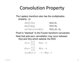
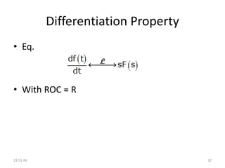
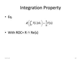
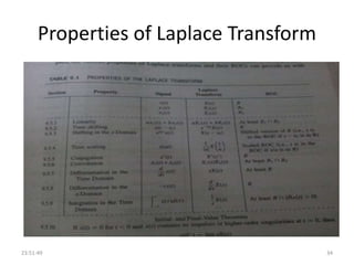
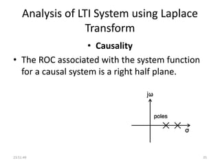
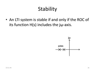
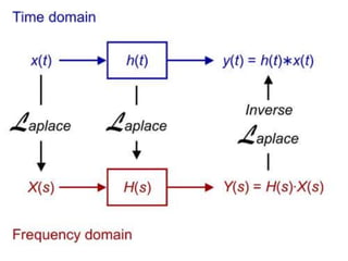
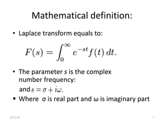
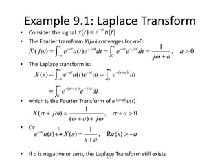
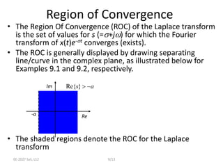
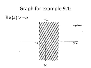
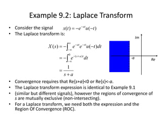
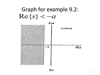
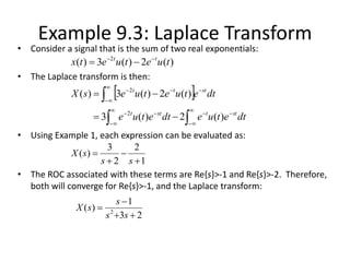
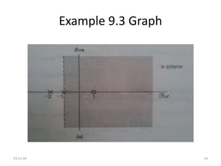
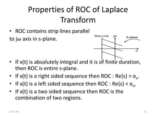
The document discusses the Laplace transform, which converts a function of time into a function of a complex frequency variable. It covers definitions, types (unilateral and bilateral), mathematical expressions, regions of convergence (ROC), properties, and examples of applications including inverse transformations and system analysis. Key characteristics about stability and causality of linear time-invariant (LTI) systems are also outlined.

1. LAPLACE TRANSFORM
CREATED BY:
BASSIT A. GOLRA
23:51:49 1

2. Laplace Transform
• Definition:
It takes function of a positive real
variable t (time) to a function of a complex
variable s ( complex frequency).
• Irrespective of whether stable or unstable
system
Source:
https://en.wikipedia.org/wiki/Laplace_transform
23:51:49 2

3. 23:51:49 3

4. Laplace Continued …
• For continues time we use Laplace transform.
• For discrete time we use Z-Transform
23:51:49 4

5. Laplace Continued …
• There are two types of Laplace transform:
i) Unilateral Laplace transform
ii) Bilateral Laplace transform
23:51:49 5

6. Unilateral Laplace
• Unilateral Laplace Transform limits from zero
to positive infinity ( 0 to ∞ )
Bilateral Laplace
 Bilateral Laplace transform limits from minus
infinity to positive infinity ( -∞ to ∞ )
• Note: we will discuss Unilateral transform only
23:51:49 6

7. Mathematical definition:
• Laplace transform equals to:
• The parameter s is the complex
number frequency:
and
 Where σ is real part and ω is imaginary part
23:51:49 7

8. 8/13
Example 9.1: Laplace Transform
• Consider the signal
• The Fourier transform X(jw) converges for a>0:
• The Laplace transform is:
• which is the Fourier Transform of e-(s+a)tu(t)
• Or
• If a is negative or zero, the Laplace Transform still exists
)()( tuetx at

0,
1
)()(
0


 





a
aj
dteedtetuejX tjattjat
w
w ww











0
)(
0
)(
)()(
dtee
dtedtetuesX
tjta
tasstat
ws
0,
)(
1
)( 

 a
ja
jX s
ws
ws
as
as
sXtue
L
at



}Re{,
1
)()(

9. EE-2027 SaS, L12 9/13
• The Region Of Convergence (ROC) of the Laplace transform
is the set of values for s (=s+jw) for which the Fourier
transform of x(t)e-st converges (exists).
• The ROC is generally displayed by drawing separating
line/curve in the complex plane, as illustrated below for
Examples 9.1 and 9.2, respectively.
• The shaded regions denote the ROC for the Laplace
transform
Region of Convergence
Re
Im
-a
as }Re{

10. Graph for example 9.1:
23:51:49 10
as }Re{

11. Example 9.2: Laplace Transform
• Consider the signal
• The Laplace transform is:
• Convergence requires that Re{s+a}<0 or Re{s}<-a.
• The Laplace transform expression is identical to Example 9.1
• (similar but different signals), however the regions of convergence of
s are mutually exclusive (non-intersecting).
• For a Laplace transform, we need both the expression and the
Region Of Convergence (ROC).
)()( tuetx at
 
as
dte
dttueesX
tas
stat











1
)()(
0
)(
Re
Im
-a

12. Graph for example 9.2:
12
as }Re{

13. Example 9.3: Laplace Transform
• Consider a signal that is the sum of two real exponentials:
• The Laplace transform is then:
• Using Example 1, each expression can be evaluated as:
• The ROC associated with these terms are Re{s}>-1 and Re{s}>-2. Therefore,
both will converge for Re{s}>-1, and the Laplace transform:
)(2)(3)( 2
tuetuetx tt 

 













dtetuedtetue
dtetuetuesX
sttstt
sttt
)(2)(3
)(2)(3)(
2
2
1
2
2
3
)(




ss
sX
23
1
)( 2



ss
s
sX

14. Example 9.3 Graph
23:51:49 14

15. Properties of ROC of Laplace
Transform
• ROC contains strip lines parallel
to jω axis in s-plane.
• If x(t) is absolutely integral and it is of finite duration,
then ROC is entire s-plane.
• If x(t) is a right sided sequence then ROC : Re{s} > σo.
• If x(t) is a left sided sequence then ROC : Re{s} < σo.
• If x(t) is a two sided sequence then ROC is the
combination of two regions.
23:51:49 15

16. Common transform pairs
23:51:49 16
( )f t ( ) [ ( )]F s L f t
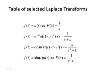
1 or ( )u t 1
s
T-1
t
e  1
s 
T-2
sin tw
2 2
s
w
w
T-3
cos tw
2 2
s
s w
T-4
sint
e t
w
2 2
( )s
w
 w 
T-5*
cost
e t
w
2 2
( )
s
s

 w

 
T-6*
t
2
1
s
T-7
n
t 1
!
n
n
s 
T-8
t n
e t
1
!
( )n
n
s  

T-9
( )t 1 T-10
*Use when roots are complex.

17. Table of selected Laplace Transforms
23:51:49 17
1
1
)()()sin()(
1
)()()cos()(
1
)()()(
1
)()()(
2
2








s
sFtuttf
s
s
sFtuttf
as
sFtuetf
s
sFtutf
at

18. Inverse Laplace transform
• The signal x(t) is said to be the inverse Laplace
transform of X(s). It can be shown that
• where c is a constant chosen to ensure the
convergence of the first
23:51:49 19

19. Inverse Laplace Transforms:
• When a differential equation is solved by Laplace
transforms, the solution is obtained as a function
of the variable s. The inverse transform must be
formed in order to determine the time response.
• The simplest forms are those that can be
recognized within the tables and a few of those
will now be considered.
• If inverse Laplace transform is complicated we
use partial fraction
23:51:49 20

20. Example. Determine the inverse
transform of the function below.
2
5 12 8
( )
3
F s
s s s
  

23:51:49 21
3
( ) 5 12 8 t
f t t e
  

21. Example. Determine the inverse
transform of the function below.
2
200
( )
100
V s
s


23:51:49 22
2 2
10
( ) 20
(10)
V s
s
 
  
 
( ) 20sin10v t t

22. Example. Determine the inverse
transform of the function below.
2
8 4
( )
6 13
s
V s
s s


 
23:51:49 23
When the denominator contains a quadratic, check the roots. If they
are real, a partial fraction expansion will be required. If they are
complex, the table may be used. In this case, the roots are
1,2 3 2s i  
2
2 2 2
2
2 2
6 13
6 (3) 13 (3)
6 9 4
( 3) (2)
s s
s s
s s
s
 
    
   
  

23. 2 2 2 2
2 2 2 2
8( 3) 4 24
( )
( 3) (2) ( 3) (2)
8( 3) 10(2)
( 3) (2) ( 3) (2)
s
V s
s s
s
s s
 
 
   

 
   
23:51:49 24
3 3
( ) 8 cos2 10 sin 2t t
v t e t e t 
 

24. Properties of Laplace Transforms
• Linearity
• Scaling in time
• Time shift
• “frequency” or s-plane shift
• Multiplication by tn
• Integration
• Differentiation
23:51:49 25

25. Linearity Property
23:51:49 26
With ROC containing R1∩R2

26. Time-Scaling Property
• Time domain scaling ⇔
frequency domain scaling
Example:
23:51:49 27
  






a
s
a
atL F
1
}{f
  22
4
2
)()2sin(
w
w
w


s
tutL
With ROC R1=R/a

27. Time Shifting
• If F (s) is the Laplace Transforms of f (t), then
• Example:
23:51:49 28
  )()()( sFeatuatfL as

as
e
tueL
s
ta




10
)10(
)}10({
With ROC =R

28. Frequency Shift
• If F (s) is the Laplace Transforms of f (t), then
23:51:49 29
)()}({ asFtfeL at

With ROC =R + Re{a}.

29. Multiplication by tn
• Eq.
• Example:
23:51:49 30
)()1()}({ sF
ds
d
tftL n
n
nn

1
!
)
1
()1(
)}({



n
n
n
n
n
s
n
sds
d
tutL
With ROC = R

30. Convolution Property
23:51:49 31

31. Differentiation Property
23:51:49 32
• Eq.
• With ROC = R

32. Integration Property
• Eq.
• With ROC= R ∩ Re{s}
23:51:49 33

33. Properties of Laplace Transform
23:51:49 34

34. Analysis of LTI System using Laplace
Transform
• Causality
• The ROC associated with the system function
for a causal system is a right half plane.
23:51:49 35

35. Stability
• An LTI system is stable if and only if the ROC of
its function H(s) includes the jῳ-axis.
23:51:49 36

36. Thanks!!
23:51:49 37