Download as PDF, PPTX


![Sunghyon Kyeong (Yonsei Univ) Introduction to Neuroimaging: Methods and Preprocessing steps p 37
Example
IB
=
?
IA
=
1
VA
=
1 VB
=
2
IA
=
1
VA
=
4
IB
=
?VB
=
2
Template
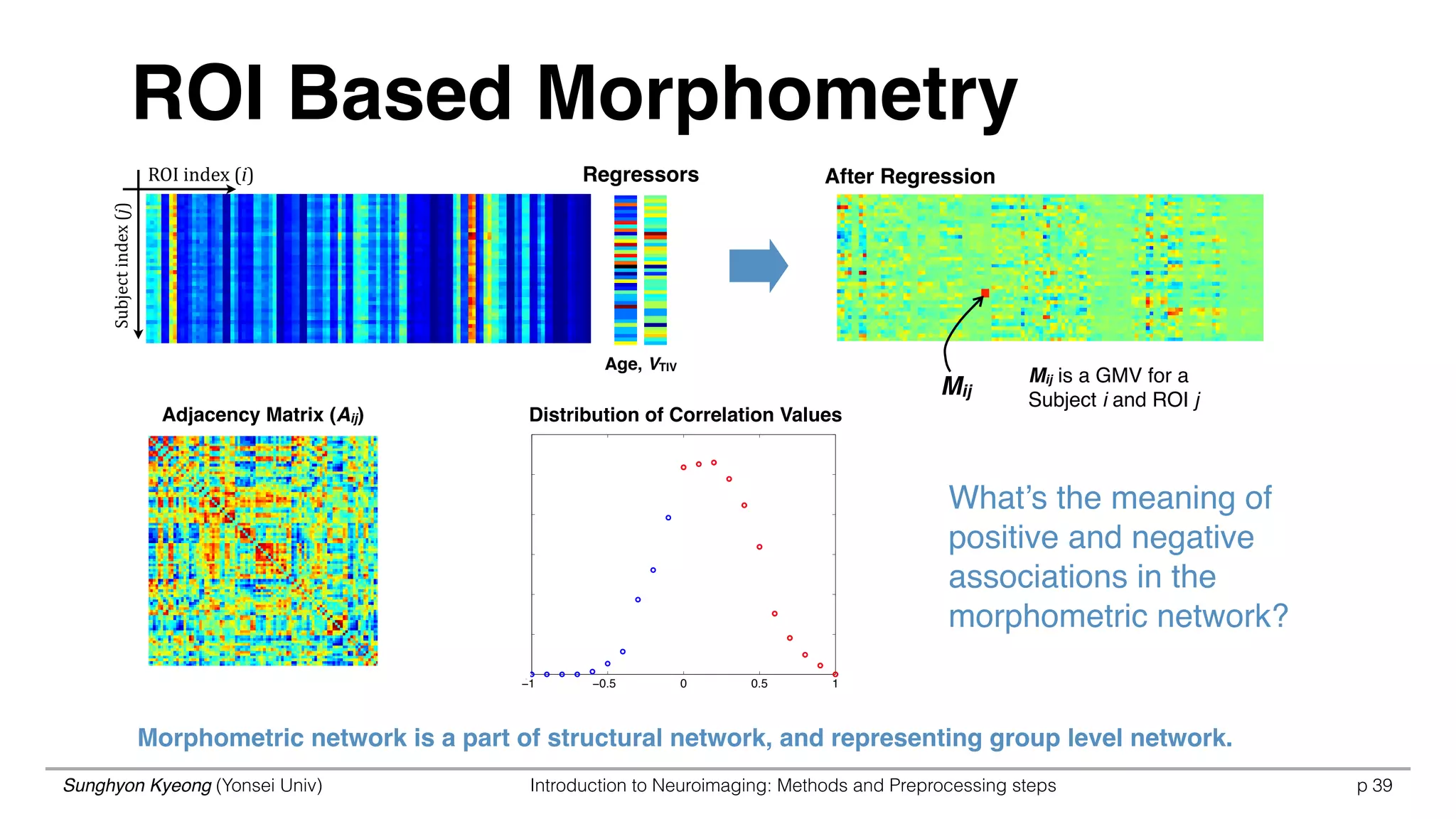
Signal intensity ensures that total amount of GM in a subject’s temporal lobe is the
same before and after spatial normalisation and can be distinguished between subjects
Template
IB = 1 × [1 / 2] = 0.5
IB = 1 × [4 / 2] = 2
Modulation
ModulationNormalisation
Normalisation
IB = IA × [VA / VB]
Larger Brain
Smaller Brain](https://image.slidesharecdn.com/tutorialfmri0neuroimagingmethods-150510110847-lva1-app6892/75/Introduction-to-Neuroimaging-37-2048.jpg)


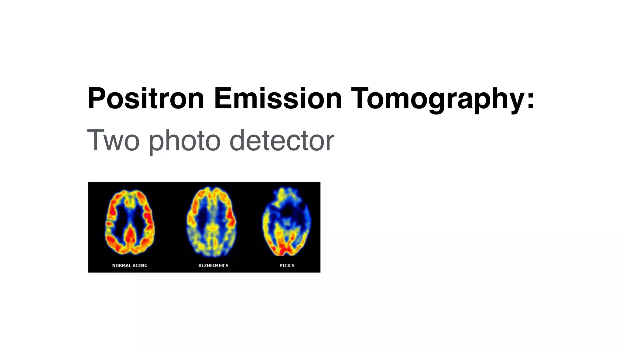
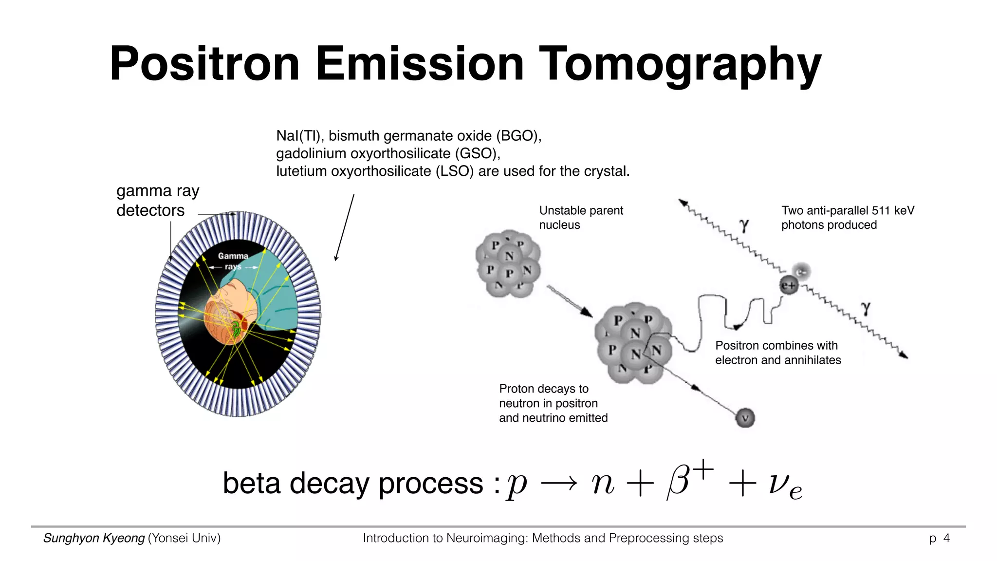
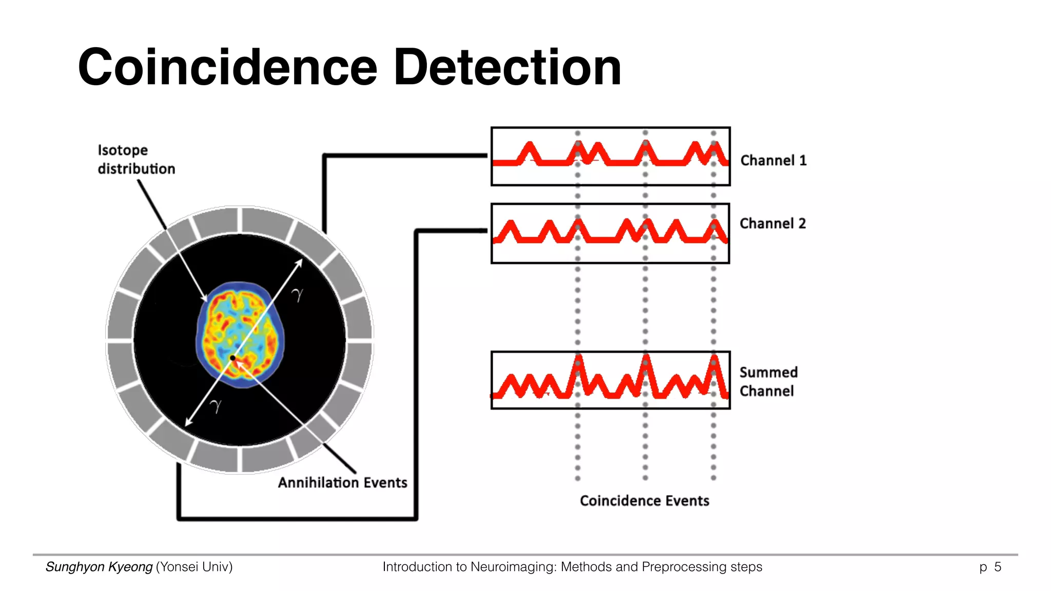
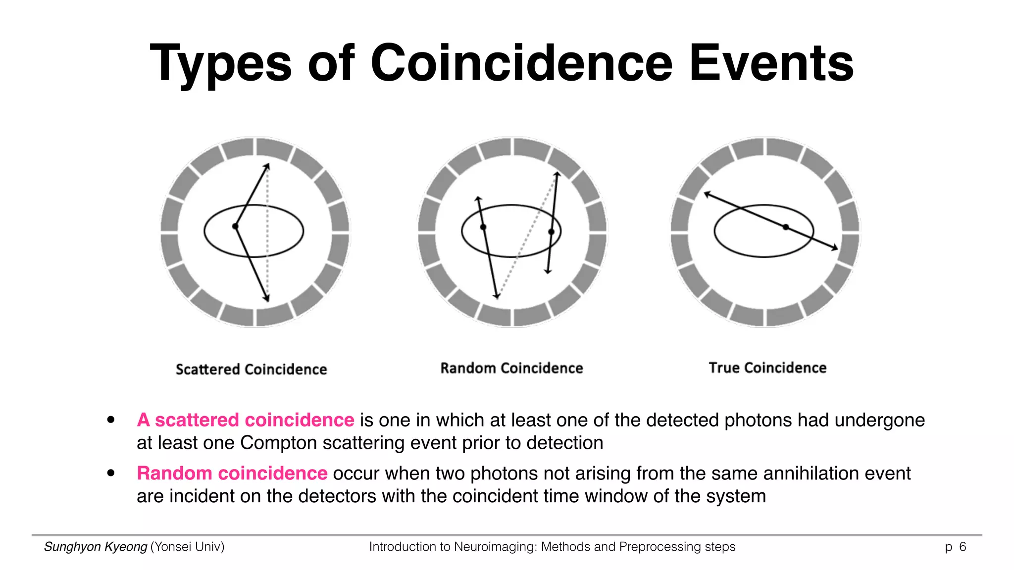
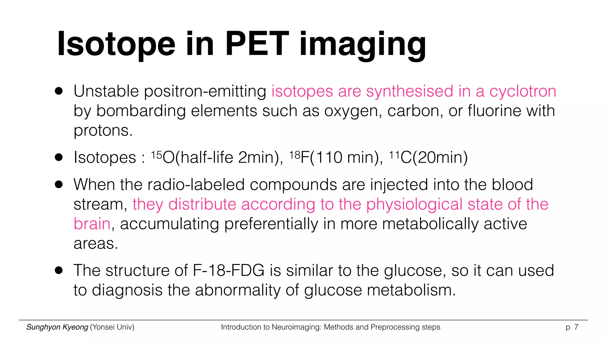
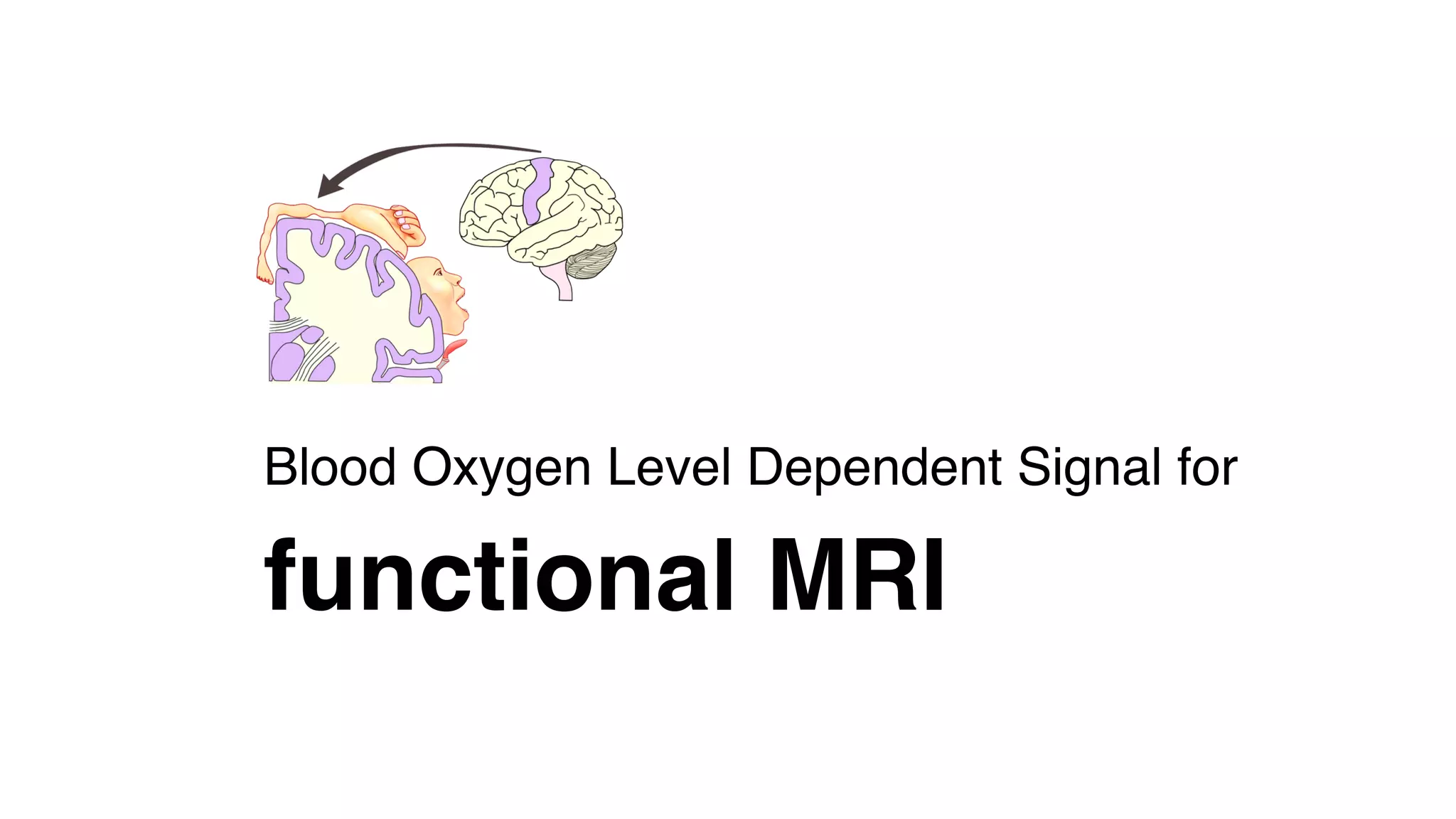
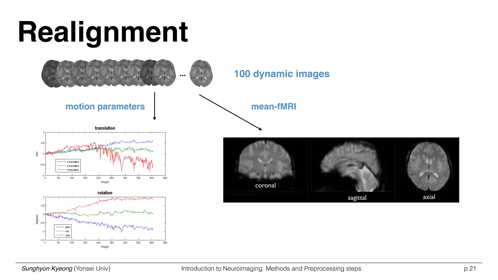
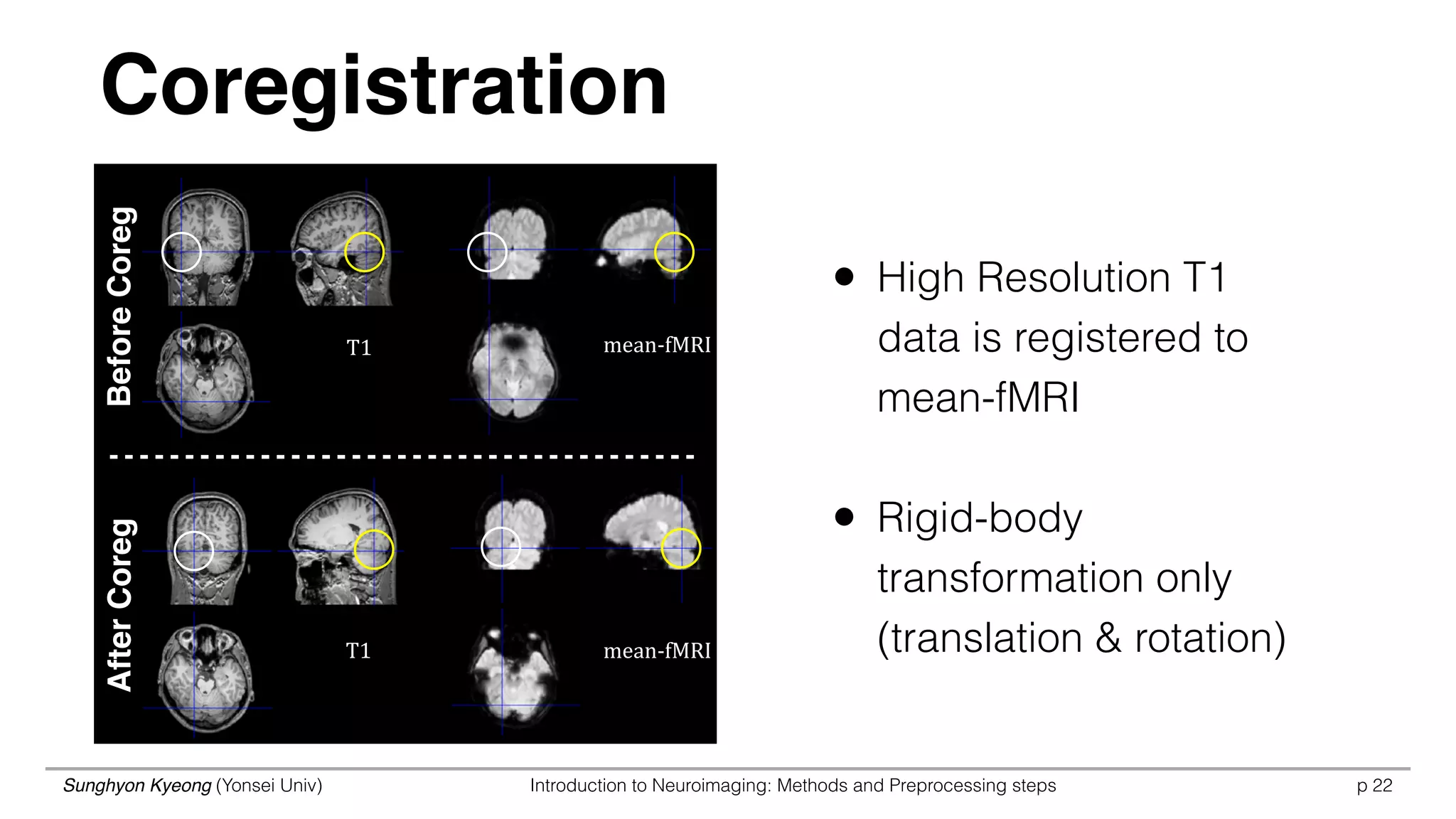
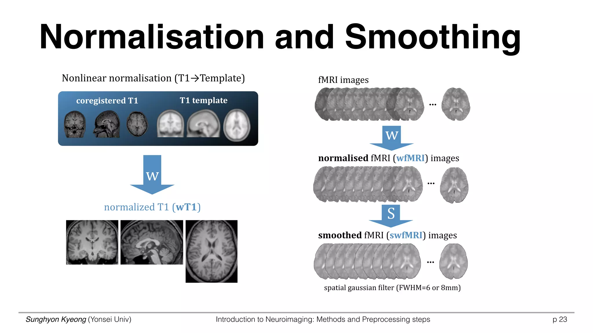
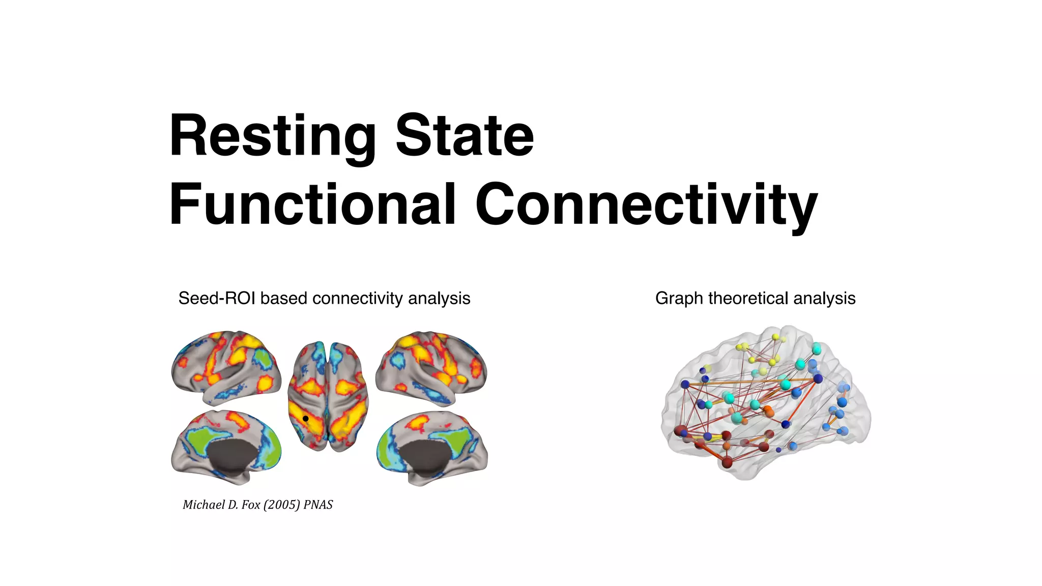
The document provides an introduction to neuroimaging techniques, specifically focusing on PET, fMRI, VBM, and DTI methods. It outlines the principles of signal generation, preprocessing steps, and the detection mechanisms for different imaging modalities, including the effects of blood oxygen levels on fMRI signals. Additionally, it covers the processes of spatial and temporal preprocessing, functional connectivity, and the construction of morphometric brain networks.