This document is a doctoral thesis submitted by Manuela P. Feilner to the Department of Microtechnology at EPFL in 2002. The thesis proposes using statistical wavelet analysis methods for functional magnetic resonance imaging (fMRI) of the brain. Chapter 1 introduces the motivation and contributions of the thesis. Chapter 2 provides background on fMRI and image acquisition techniques. Subsequent chapters develop statistical analysis methods using wavelet transforms and apply them to analyze real fMRI data to identify brain activation patterns. The goal is to improve detection of activated regions compared to existing real-space methods.


![Chapter 1
Introduction
1.1 Motivation
The brain is the most complex organ of a human being. Some authors have even claimed
that it is the most complex entity in the universe. For several thousand years humans—
philosophers, poets, musicians and more recently scientists—have been trying to disclose
the secret of the function of the brain. The question is: what is the relationship between
the brain and mental functions, including perception, memory, thought and language ?
Today, we are in the exciting phase of starting to understand how the brain works. A
crucial role is played here by imaging techniques such as functional Magnetic Resonance
Imaging (fMRI). Several brain areas which are activated by physiological stimuli have
already been discovered. Now, more diffuse connections are being investigated. Scientists
are starting to study neural correlates of many emotional states. One example, which
recently made headlines, is the investigation of the neural basis of romantic love. The
activity in the brains of 17 subjects who were deeply in love was scanned using fMRI
while they viewed pictures of their partners. It was compared with the activity produced
by viewing pictures of three friends of similar age, sex and duration of friendship as
their partners [12]. The authors found a unique network of areas which is responsible for
evoking this affective state.
Another example is the perception of music. Music plays a crucial role in every culture.
It has been discovered that different types of music—or composers—affect different areas
of the brain.
Another strong incentive to monitor the function of the brain is the search for better
diagnostic tools and treatment planning. There are several neurological diseases such as
epilepsy for which the last treatment, when the patient does not respond to medication, is
neurosurgery. To minimize the potential risk of such an invasive treatment, neurosurgery
relies on a precise delineation of the structural and functional aspects of the brain. fMRI](https://image.slidesharecdn.com/0eba55bf-42a7-4963-8f0c-60b852f024ac-160911124222/85/feilner0201-11-320.jpg)


![Chapter 2
Functional Magnetic Resonance
Imaging (fMRI)
2.1 A brief historical view
Before functional Magnetic Resonance Imaging (fMRI), there was only one way to access
the functionality of the human brain: One had to study the brains of ill people after
they had died and compare them to healthy ones. This way many brain discoveries were
made from the examination of injuries or malformations. In 1861, the French surgeon
Paul Broca had a patient who could speak only one sound: “tan”, after suffering a stroke.
Following the death of this patient, Broca examined his brain and discovered a damaged
spot on the front left side. He suspected that this area controlled speaking ability [23].
He was right. “Broca’s area” was the first recognized link between brain function and
its localization.
In 1890 C.W. Roy and C.S. Sherrington, in their paper On the regulation of blood
supply of the brain, suggested that neural activity was accompanied by a local increase
in cerebral blood flow [119]. The possibility of imaging this effect started in 1946, when
Felix Bloch at Stanford, studying liquids, and Edward Purcell at Harvard, studying
solids, described—independently of each other—the nuclear magnetic resonance phe-
nomenon [19, 112]. They discovered that certain substances are able to absorb and emit
radiofrequency electromagnetic radiation, when they are placed in a magnetic field. The
absorption and emission was related to the substance being studied. This new technique,
Nuclear Magnetic Resonance (NMR), was used for chemical and physical molecular anal-
ysis between 1950 and 1970. Bloch and Purcell were awarded the Nobel prize for physics
in 1952 for this discovery, but it was not until 1973 that NMR was used to generate
images from inside the body. It was in 1971, when Raymond V. Damadian showed that
the nuclear magnetic relaxation times of healthy and cancerous tissues differed, that sci-](https://image.slidesharecdn.com/0eba55bf-42a7-4963-8f0c-60b852f024ac-160911124222/85/feilner0201-15-320.jpg)
![6 Chapter 2. Functional Magnetic Resonance Imaging (fMRI)
entists started to consider magnetic resonance for the detection of disease [40]. In 1973,
a chemist, Paul Lauterbur, improved the technique significantly. He succeeded in getting
from the one-dimensional spatial representation to a complete two-dimensional scan [87].
But the human body is three-dimensional and it was Peter Mansfield who developed the
three-dimensional technique [96]. The basis of the current Magnetic Resonance Imag-
ing (MRI) technique was finalized by Anil Kumar, Dieter Welti, and Richard R. Ernst
at ETH Z¨urich [83]. They applied Fourier reconstruction techniques to encode spatial
information in the phase and frequency of the NMR signal.
MRI is tuned to image the hydrogen nuclei of water molecules. In functional MRI,
Blood Oxygenation Level Dependent (BOLD) effects are measured for mapping brain
functions. Until 1990 there was no non-invasive way of measuring the flow of blood
in cortical areas. Ogawa and Lee at the AT & T Bell Laboratories and Turner at
the National Institutes of Health (NIH), working independently on laboratory animals,
discovered that the oxygenation level of blood acts as a contrast agent in MR images [108,
142]. This discovery led to the technique of fMRI as it is in use today [41, 98].
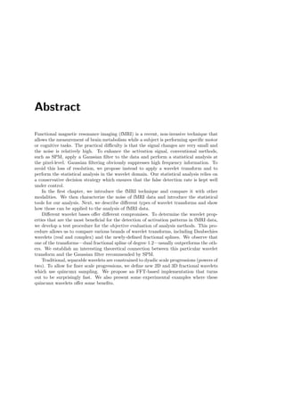
In the past few years, the interest in fMRI has increased continuously, as indicated
by the number of papers published in this area (cf. Figure 2.1).
96 97
# papers
for fMRI
150
50
-1992 93-94 95 98 99 20012000 year
100
Figure 2.1: Papers published in the last few years related to the subject of functional Magnetic
Resonance Imaging (from the INSPEC database only).](https://image.slidesharecdn.com/0eba55bf-42a7-4963-8f0c-60b852f024ac-160911124222/85/feilner0201-16-320.jpg)
![2.2. Principle of Magnetic Resonance Imaging 7
2.2 Principle of Magnetic Resonance Imaging
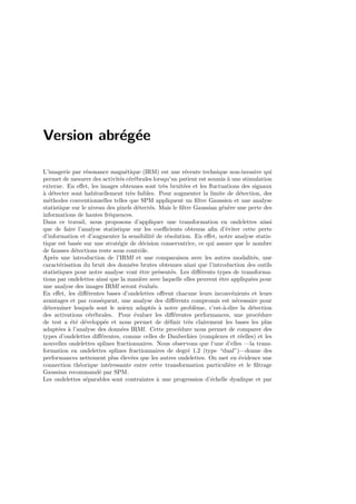
A modern MRI scanner, from which we get our fMRI images, is depicted in Figure 2.2.
In this section we describe briefly the underlying principles of fMRI [6, 14, 53, 63, 24, 90,
139, 126].
Figure 2.2: Example of a magnetic resonance scanner with a magnet of 1.5 tesla. It belongs to
the Siemens “MAGNETOM Symphony Maestro Class” range [127].
2.2.1 Relaxation phenomena
The MR signal in its classical clinical use is predominantly a signature from the protons
of tissue water in humans. The technique of Nuclear Magnetic Resonance (NMR) is
based on the fact that atoms of hydrogen H1
, but also elements like sodium (Na23
) and
phosphorus (P31
), have a nuclear spin, which is proportional to the angular momentum
of the nucleus (the proportionality constant is the gyromagnetic ratio). In general, atoms
which have an odd atomic number or an odd atomic weight have a resulting nuclear spin.
Such a nucleus can be seen as a rotating electrically charged object causing a magnetic
moment. In human tissue, we deal with a large number of such nuclei. At a macroscopic
level these magnetic dipoles form an ensemble and the sum of their magnetic moments,
the nuclear magnetization, is equal to zero provided there is no exterior magnetic field.
When such nuclei are immersed in a static magnetic field B0 = (0, 0, B0) in the z-
direction, the total magnetic moment, the nuclear magnetization M, is oriented in the
direction of the applied field B0 (parallel or anti-parallel heading). In MRI a very strong](https://image.slidesharecdn.com/0eba55bf-42a7-4963-8f0c-60b852f024ac-160911124222/85/feilner0201-17-320.jpg)
![2.2. Principle of Magnetic Resonance Imaging 9
x
y
z
xyM
M z
x
y
z
xyM
M z
xyM
M z
x
y
z
Figure 2.4: The decrease of the transverse magnetization component Mxy of the spins in a
molecule, which is related to the transverse relaxation time T2.
of the phase. The space coding of two orthogonal axes is usually achieved by applying
these two methods.
The imaging effect of the contrast parameters T1 and T2 can be suppressed or en-
hanced in a specific experiment by another set of parameters, such as repetition time
(TR), echo time (TE), and flip angle (α) [90]. This distinction allows certain structural
components to be emphasized. Water for example has very similar T1 and T2 times.
In cerebrospinal fluid (CSF) T1 is larger than T2, and in white matter the difference is
even greater. Therefore, T1-weighted imaging is an effective method to obtain images of
a good anatomical definition and T2-weighted imaging is a sensitive method for disease
detection, since many disease states are characterized by a change of the tissue’s T2 value.
Figure 2.5 shows an example of T1- and T2-weighted images.
a) b)
Figure 2.5: a) T1-weighted head image. b) T2-weighted head image: the tumor is more visible.](https://image.slidesharecdn.com/0eba55bf-42a7-4963-8f0c-60b852f024ac-160911124222/85/feilner0201-19-320.jpg)
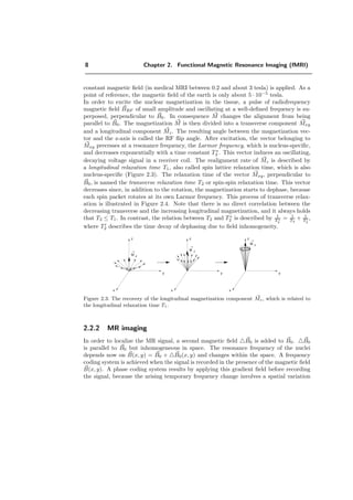
![10 Chapter 2. Functional Magnetic Resonance Imaging (fMRI)
2.2.3 Fast MR imaging
fMRI of a human brain, must be performed rapidly. One reason is that the movements of
the patient increase with time; another is that the images of the whole volume of the brain
should be acquired within the same activation condition. Furthermore, the patient can
perform most of the cognitive tasks of interest only for a few minutes without habituation
or fatigue. Two such faster methods are Fast Low Angle SHot (FLASH) and EchoPlanar
Imaging (EPI). FLASH uses a small interval between the RF pulses to reduce the flip
angle and therefore also T1 [74], while EPI uses smaller RF pulses that excite only a
fraction of the protons, which reduces relaxation time. EPI requires a strong gradient
field, which was not available when FLASH was invented. EPI, invented by Mansfield
et al. [133], acquires a complete image in less than 100 ms. It is currently a widely
deployed method. However, this technique suffers more than others from distortion and
signal loss arising from magnetic field inhomogeneities in the brain. Nevertheless the
experiments with real data described in this thesis were all performed with EPI, since it
is at present the most commonly used technique. Further description of (noise) artifacts
of rapid imaging methods can be found in Section 3.3.1.
2.3 BOLD contrast in fMRI
In fMRI experiments, we alternate between an activation state where the patient per-
forms a certain task and a rest state where no task is performed. The task involves
changes of neuronal activation during an activation state in the brain. With fMRI, we
cannot measure directly the neuronal activities, but their related effects. Ogawa [107] and
Turner [142], working with laboratory animals, observed independently in 1990 that MRI
image contrast changes around the blood vessels could be obtained by the modification of
the oxygenation state of the blood. This effect arises from the fact that deoxyhemoglobin
is more paramagnetic than oxyhemoglobin, which itself has almost the same magnetic
susceptibility as tissue. Thus deoxyhemoglobin can be seen as nature’s own contrast
agent. Neuronal activity is related to changes of the oxygenation state because neurons
need oxygen to function, since they are cells. This oxygen is carried to the neurons by
oxyhemoglobin within the red blood cells, the erythrocytes. The oxygen uptake by the
neurons causes a deoxygenation of the oxyhemoglobin, which becomes deoxyhemoglobin.
In addition, neurons need glycogen for their metabolic processes during electrical activity,
which is also carried by the erythrocytes. The need for oxygen and glucose of the neurons
during electrical activity causes an increased blood flow and perfusion in the capillar-
ies. But the oxygen consumption increases only slightly during activation, therefore the
relation between oxyhemoglobin and deoxyhemoglobin changes. This relative decrease
in the concentration of paramagnetic deoxyhemoglobin indicates activation, which can
be measured by the fMRI method. Since the resulting image contrast depends on the
oxygen content of the blood, this method is called Blood Oxygenation Level Dependent](https://image.slidesharecdn.com/0eba55bf-42a7-4963-8f0c-60b852f024ac-160911124222/85/feilner0201-20-320.jpg)
![2.4. Different imaging modalities 11
(BOLD) contrast [110, 53].
There is also a more recent alternative contrast mechanism for visualizing functional
activation in the brain that provides direct measurement of cerebral blood flow (CBF)
using MRI. This technique, called arterial spin labeled (ASL) perfusion MRI, utilizes
electromagnetically labeled arterial blood water as endogenous tracer for measuring CBF
[45, 49].
Perfusion contrast has some advantage over the BOLD technique. In particular, it im-
proves the independence of the observations in time under the hypothesis that no ac-
tivation is present, whereas BOLD-data signals can be correlated. However, perfusion
contrast has a poorer temporal resolution and is less sensitive than the BOLD contrast
method [4].
2.4 Different imaging modalities
We will now briefly discuss the two other competing functional imaging methods, PET
(cf. Figure 2.6) and SPECT, which are older than fMRI.
Figure 2.6: Example of a Positron Emission Tomograph. It belongs to the Siemens “ECAT
EXACT” range and is the most widely used PET scanner [127].
2.4.1 Positron Emission Tomography (PET)
The history of PET began in the early 1950s, when the medical imaging possibilities of
a particular class of radioactive substances were first realized. By the mid-1980s, PET
had become a tool for medical diagnosis and for dynamic studies of human metabolism.](https://image.slidesharecdn.com/0eba55bf-42a7-4963-8f0c-60b852f024ac-160911124222/85/feilner0201-21-320.jpg)
![12 Chapter 2. Functional Magnetic Resonance Imaging (fMRI)
PET imaging begins with the injection of a metabolically active tracer into the pa-
tient. The tracer is built by a biological molecule that carries a positron-emitting isotope
(known as the radioactive tag), such as 11
C (carbon-11), 18
F (fluorine-18), 15
O (oxygen-
15) or 13
N (nitrogen-13), which have short decay times. Over a few minutes, the isotope
accumulates in an area of the body for which the carrier molecule has an affinity. For
example, glucose labeled with 11
C accumulates in the brain or in tumors where glucose
is used as the primary source of energy. The radioactive nuclei then decay by positron
emission. Thus PET provides images of biochemical functions, depending upon the type
of molecule that is radioactively tagged. The emitted positron combines with an electron
almost instantaneously, and these two particles experience the process of annihilation.
The energy associated with the masses of the positron and electron is divided equally
between two photons that fly away from one another at a 180◦
angle. These high-energy
γ-rays emerge from the body in opposite directions and are detected by an array of cir-
cular γ-ray detectors that surround the body of the patient [24]. These detectors have
a series of scintillation crystals, each connected to a photomultiplier tube. The crystals
convert the γ-rays to photons, which the photomultiplier tubes convert to electrical sig-
nals and amplify. These electrical signals are then processed by the computer to generate
images. Figure 2.7 shows such an image.
Figure 2.7: PET image from a slice of the human brain.
There are some limitations of PET. Higher order cognitive processes increase regional
Cerebral Blood Flow (rCBF) by only about 5%. This small amount can only be detected
when multiple subjects are used and this relates to the problem of anatomical variation
between the subjects. Another limitation are the spatial and temporal resolutions, which
are lower than for fMRI, i.e., 3 mm and 60 s, respectively, compared to ∼ 1.5 mm and 100](https://image.slidesharecdn.com/0eba55bf-42a7-4963-8f0c-60b852f024ac-160911124222/85/feilner0201-22-320.jpg)
![2.5. Description of typical fMRI data 13
ms for fMRI. PET scanners are also less available than fMRI scanners, since they must
be located near a cyclotron device that produces the short-lived radioisotopes used in the
technique. Further advantages of fMRI over PET are lower costs, reduced invasiveness,
structural and functional information, and a larger signal-to-noise ratio. On the other
hand, PET shows a greater sensitivity in certain aspects, such as soft auditory and overt
speech stimulation [124, 79], since the loud noise of the fMRI scanner can interfere with
the auditory tasks. (Today, however, good hearing protection is available, so that more
and more auditory tasks can also be done with an fMRI scanner.) When performing
an experiment with PET and fMRI, the activation zones detected were mostly identical.
However the activation zones are slightly larger in the case of fMRI, probably due to the
better signal-to-noise ratio.
2.4.2 Single Photon Emission Computed Tomography (SPECT)
Single Photon Emission Computed Tomography (SPECT) is a technique similar to PET.
But the radioactive substances used in SPECT (xenon-133, technetium-99, iodine-123)
have longer decay times than those used in PET, and emit single instead of double γ-rays.
SPECT can provide information about blood flow and the distribution of radioactive
substances in the body. Its images have less sensitivity and are less detailed than PET
images, but the SPECT technique is less expensive than PET. Also SPECT centers
are more accessible than PET centers because they do not have to be located near a
cyclotron.
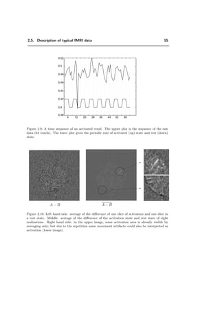
2.5 Description of typical fMRI data
The first step in an fMRI experiment is the set-up of the experimental design by a
neurologist. The task succession must be chosen in order to find the relation between
the brain activation and a certain motor or cognitive task and to filter out inappropriate
actions. For example, a cognitive task meight be listening to a specific sound or to music
or viewing a screen displaying different pieces of information or images.
During the fMRI experiment a volunteer lies in an MRI scanner, his head fixed with
a helmet-like device to avoid strong movement artifacts. A sequence of images of the
volunteer’s brain is acquired while he performs the specified tasks. The spatial resolution
of the obtained images (slices) is typically 2–3 mm and the thickness of one slice is usually
3–10 mm. An example of an acquired volume is given in Figure 2.8. Using the fast EPI
technique, 3–10 images per second can be acquired [63].
The experimental design can be based on a block paradigm or an event-related fMRI,
which we will explain below. All of the real data investigated in this thesis are based on
the block paradigm. We received our data through collaborations with the Inselspital
Bern and the Hˆopital Cantonal Universitaire de Gen`eve (HCUG).](https://image.slidesharecdn.com/0eba55bf-42a7-4963-8f0c-60b852f024ac-160911124222/85/feilner0201-23-320.jpg)
![14 Chapter 2. Functional Magnetic Resonance Imaging (fMRI)
. .
. . . .
. .
. . . .
. .
Figure 2.8: Example of some slices of a volume of raw data. The inplane number of pixels is
128 × 128, the number of slices in a volume is 30. Thus the resolution along the z-axis is lower
than in the xy-plane.
2.5.1 Block paradigm
In the case of the block paradigm, fMRI data consist of repetitions of alternating A and
B epochs. Symbol A stands for the brain volume with activation (the subject performs a
certain task) and B for the brain volume in the rest state. An epoch contains a sequence
of several repetitions under the same condition. A cycle contains one epoch under each
condition [17]:
A A A A B B B B
cycle
A A A A
epoch
B B . . .
A time sequence of one voxel of an activated area is shown in Figure 2.9. It is
obvious that a lot of noise is present in the data; the underlying signal, which should
follow the periodic activation pattern, is hardly recognizable even though the voxel is
taken from a strongly activated region (upper limit of the signal-to-noise ratio). The
difference image of two slices (A–B) is shown in Figure 2.10. The amount of noise makes
it almost impossible to detect any activation with only one realization. Thus the fMRI
algorithms are based on averaging over several realizations. Some activation zones are
visible by averaging only, see Figure 2.10. However, the limiting factor in averaging is
the volunteer’s ability to stay that long time in the scanner and to perform identical
tasks without moving insight the scanner. Even with few repetitions the images may be
corrupted by movement artifacts.
2.5.2 Event-related fMRI
An alternative to the block paradigm is the Event-Related experiment protocol (ER-
fMRI), which involves a different stimulus structure. Event-related protocols are charac-](https://image.slidesharecdn.com/0eba55bf-42a7-4963-8f0c-60b852f024ac-160911124222/85/feilner0201-24-320.jpg)
![16 Chapter 2. Functional Magnetic Resonance Imaging (fMRI)
terized by rapid, randomized presentation of stimuli. This is analogous to the technique
of Event-Related Potentials (ERPs), which uses electric brain potentials that are mea-
sured by electrodes on the scalp or implanted in the skull [115]. The disadvantage of
ERPs is their bad spatial information, although their time resolution is excellent.
The event-related experiment combines the advantage of time information of ERP and
the advantage of good spatial resolution of fMRI. The time information is important
for determination of the Hemodynamic Response Function (HRF), which represents the
regional BOLD effect signal change after a short stimulus. The time between two stimuli
(Inter-Stimulus Interval (ISI)) can be chosen randomly. This has the advantage that the
volunteer does not get used to the experiment, which implies that the HRF does not
change its shape or decrease in amplitude. This is necessary in order to be able to sum
over several realizations [27]. Other advantages, such as the possibility of post hoc cate-
gorization of an event, are reported in [75, 80, 149]. However, for steady-state analysis,
the block paradigm is still the most effective one.
2.6 Preprocessing
We call preprocessing all processes which are prior to the statistical analysis and the
possible image transformations of the data.
In the case of the block paradigm, the common practice is to omit the first volume of
each block (Figure 2.11) or to shift the paradigm by one or even two volumes. This is
because the volumes at the beginning of a block contain a transition signal that would
make the steady-state analysis more difficult. Another possibility is to keep this first
transition measurement by introducing a hemodynamic function in the model [11, 113].
We restricted ourselves to the first approach as presented in Figure 2.11, which was
proposed by our collaborators and enabled us to compare the methods. Also a hypothesis
need only be made about the length of the transition signal and not about the shape of
the hemodynamic function.
A A A A B B B B A A A A B B B B . . .
Figure 2.11: Typical ordering of the fMRI data with suppression of the first volume.
Another very important preprocessing step is motion correction. Getting data with
the fewest possible head movements is a requisite. But head motions cannot be com-
pletely avoided. A movement of one tenth of a voxel may produce 1–2% signal changes,
which is not negligible. In comparison, fMRI BOLD effects are very small: 1–5% signal
changes [37, 71]. This calls for the use of accurate image registration algorithms [140, 65].
The first step in registration is to determine parameter values for the transformation of
the images toward a reference image, the target image, which is often the first acquired](https://image.slidesharecdn.com/0eba55bf-42a7-4963-8f0c-60b852f024ac-160911124222/85/feilner0201-26-320.jpg)
![2.6. Preprocessing 17
image. The images are transformed by resampling according to the determined geome-
try, which is evaluated by optimizing some criterion that expresses the goodness of the
matching [8]. In order to realign our data, we used mainly the method proposed in SPM
[65], see Section 2.8. We also analyzed data realigned with the Automated Image Regis-
tration (AIR) method [153, 154]. The third realignment, which we used, is a high-quality
realignment procedure developed in our group [140]. Figure 2.12 illustrates the influence
of realignment.
a) without realignment b) with realignment
Figure 2.12: Example of the influence of realignment. The activation in the brain was caused
by a visual task. a) Detection of activation based on raw data with the algorithm developed in
this work. Some of these detected areas are caused by movement artifacts, in particular the one
on the border in the upper brain region. b) Detection of activation based on data which were
realigned with SPM99. Most of the detected areas which were caused by movement artifacts
disappear.
Sometimes it is desirable to compare the analysis of different subjects or even ana-
lyze across different subjects. In such cases spatial normalization is applied to the data
between the subjects. Subjects can even be spatially normalized according to their Eu-
clidian coordinate within a standard space [62]. The most commonly adopted coordinate
system within the brain imaging community is that described by Talairach and Tournoux
[137]. Matching here is only possible on a coarse scale, since there is not necessarily a
one-to-one mapping of the cortical structures between different brains. Consequently,
the images are smoothed prior to the matching [8].
No such processing was required in our work since we did not engage in inter-subject
studies.
Almost every fMRI scanner acquires the slices of a volume in succession. Slice timing
correction shifts each voxel’s time series so that all voxels in a given volume appear to
have been captured at exactly the same time [131].
Spatial filtering with a smoothing kernel is often applied to the data to increase the](https://image.slidesharecdn.com/0eba55bf-42a7-4963-8f0c-60b852f024ac-160911124222/85/feilner0201-27-320.jpg)
![18 Chapter 2. Functional Magnetic Resonance Imaging (fMRI)
signal-to-noise ratio. But this will only work if the activation zone is larger than the size
of the smoothing kernel. Smoothing decreases the resolution, whereas the MRI-scanner
technique is constantly upgraded to produce higher resolution data.
Global intensity normalization, also known as time normalization, is applied to the
data, when the intensities of the voxels drift over time [25, 68]. For this purpose, the mean
value of each volume in time is measured, taking only voxels above a certain threshold
into account which represents the intracerebral voxels. Then the intensities are adjusted
such that each volume has the same mean value. This treatment is more necessary for
PET data than for fMRI data, since in the first case the amount of radioactivity in
the brain can change during acquisition. Global intensity normalization can affect the
detection results when the activation is sufficiently large and very significant such that
the mean value is strongly influenced by this activation. It is therefore only useful when
there are big changes in global intensity.
The data may include slow, repetitive physiological signals related to the cardiac cycle
or to breathing. With a temporal filter, in this case a high-pass filter, these periodic
signals can be avoided. Also, scanner-related drifts are suppressed with such a filter.
2.7 An overview of fMRI postprocessing methods
By postprocessing methods, we mean the statistical analysis and possible image trans-
formations; i.e., all treatments that are used to find the activation loci. At this stage,
the data have already been preprocessed, e.g., realigned.
2.7.1 Real space methods
An early developed and still often used method is the correlation analysis introduced
by Bandettini et al. [11]. The key to this approach is the formation of the correlation
coefficient, cc, for each pixel:
cc =
N
n=1 (fi − µf ) (ri − µr)
N
n=1 (fi − µf )
2 N
n=1 (ri − µr)
2
. (2.1)
fi (i = 1 . . . N) is the time-course function at a fixed spatial location. It can be considered
to be an N dimensional vector. ri is a reference waveform or vector. This reference may
be an experimental time-course function f for some particular pixel or an average of the
f s of several experiments, which is then correlated with the time-course function f of
other pixels. Alternatively, it is a signed sequence (1 1 1 –1 –1 –1 . . . ) coding for the
paradigm [152]. µf and µr are the average values of the vectors f and r, respectively.
The value of cc always varies between +1 and −1. A threshold value TH between 0 and](https://image.slidesharecdn.com/0eba55bf-42a7-4963-8f0c-60b852f024ac-160911124222/85/feilner0201-28-320.jpg)
![2.7. An overview of fMRI postprocessing methods 19
+1 is selected and data in each pixel where
cc < TH
are rejected, i.e., set to zero. A value of 0.7 for TH is a typical threshold [11]. In order to
further distinguish between time courses, the application of additional procedures (e.g.
amplitude threshold [15] or cluster-size threshold [61]) is advantageous.
Another more powerful statistical approach is the use of a generalized linear model [100]
pioneered by Friston et al. [67] which was used for PET studies first and has then been
adapted to fMRI; it is called Statistical Parameter Mapping (SPM) and is freely available
as a software tool (SPM99). Since SPM is largely used by neurologists and is the de facto
standard in the field, we devote a whole section to this method (see Section 2.8). We
will also compare our results with the results of SPM (cf. Chapter 7).
The analyses discussed so far need prior knowledge about the succession of activation (A)
and rest state (B). Among the methods that do not require prior knowledge at all, the
earliest are Principal Component Analysis (PCA) [150] and Factor Analysis (FA) [10].
However, these do not work so well for evaluating fMRI data because the total variance
of the data is dominated not by the activation changes but by (physiological) noise which
is then partitioned into uncorrelated components [13].
Fuzzy Clustering Analysis (FCA) is another technique which is paradigm-independent,
fast and reliable [122, 55]. It attempts to find a partition of a dataset X of n feature
vectors (x1, x2, . . . , xn) by producing, for a preselected number of clusters c, c vectors in
a feature space Rp
, called cluster centroids or prototypes. They represent points around
which the data are concentrated. For each datum, a membership vector uk measures
the similarity of the point to each cluster centroid and indicates how well the point is
classified. But often, this classification suffers from the high amount of noise present in
the data. We believe that a multiresolution approach for classifying could reduce this
problem.
For completeness sake, we also mention the existence of other less popular methods that
are briefly described and compared to each other in [85]. The conclusion of this author is
that a pluralistic empirical strategy coupled formally with substantive prior knowledge
of the data set is better than employing a single method only. In [73] different soft-
ware tools for analyzing fMRI data are described and compared. These software tools
are AFNI 2.01 (Analysis of Functional NeuroImages) [38, 36]; SPM96 (Statistical Pa-
rameter Mapping) [66]; STIMULATE 5.0 [136]; Yale [128]; MEDIMAX 2.01, conceived
by the Infographics Group in 1995; FIASCO (Functional Imaging Analysis Software-
Computational Olio) [50]; MEDx 2.0, a commercial multimodality brain imaging pro-
cessing and analysis software by Sensor Systems; and FIT (Functional Imaging Toolkit)
(unpublished). The software BrainVoyager1
, a commercial software-tool conceived by
Brain Innovations B.V., offers various possibilities, such as time-course analysis of fMRI.
BrainVoyager is easier to handle than SPM96 and is thus being used more and more
1http://www.brainvoyager.de/](https://image.slidesharecdn.com/0eba55bf-42a7-4963-8f0c-60b852f024ac-160911124222/85/feilner0201-29-320.jpg)
![20 Chapter 2. Functional Magnetic Resonance Imaging (fMRI)
by medical doctors and scientists for analyzing fMRI data. The authors of SPM and
BrainVoyager are collaborating on the creation of an interface between these two image
analysis environments.
2.7.2 Wavelet methods
The use of the wavelet transform for the analysis of functional Magnetic Resonance Imag-
ing (fMRI) of the brain was pioneered by Ruttimann et al. [120]. Their statistical test
consists of a two-stage approach: first all subbands are tested with a χ2
-test globally, to
detect the presence of a signal. When the energy in the subband is too low, the subband
is discarded. In the second stage, the coefficients of the remaining subbands are thresh-
olded individually via a two-tailed z-test. These authors used orthogonal cubic-spline
wavelets.
In [116], Raz et al. perform an analysis of variance (ANOVA) in the wavelet domain by
thresholding the wavelet coefficients according to their score in a statistical test. The test-
ing is done per block. At the coarsest level, each block consists of 16 coefficients; at finer
levels the block contains all its child coefficients at those levels. They used Daubechies
least asymmetric wavelets with 8 filter coefficients, also called “symmlets” [43]. For
multiple comparisons correction, they proposed to use the False Discovery Rate (FDR),
which is much less conservative than the Bonferroni correction applied by Ruttimann et
al.
There have also been some attempts to apply wavelets to the analysis of PET data: Rut-
timann et al. [121], Unser et al. [146] and Turkheimer et al. [141]. In [141], the problem
of estimation of the spatial dimension is solved by applying the wavelet transform to each
scan of the dynamic PET sequence and then performing the kinetic modeling and statis-
tical analysis in the wavelet domain. These authors used a Translation-Invariant Discrete
Wavelet Transform (DWT-TI) introduced by [33], which does not imply a unique inverse
transform.
In another work [26, 54], the wavelet transform of fMRI time signals is used to remove
temporal autocorrelations.
In [102, 101], F. Meyer demonstrates that, with a wavelet-based estimation, a semi-
parametric generalized linear model of fMRI time-series can remove drifts in time that
cannot be adequately represented with low degree polynomials.
In [151], wavelet denoising is performed as an alternative to Gaussian smoothing. The
statistical testing (FDR) is done in the space domain. The authors chose to use the
symmetric orthonormal spline of degree α = 5.
For our part, we have also contributed to this research by extending the statistical testing
to the non stationary case [57] and by searching for objective criteria for comparing the
performance of various wavelet transforms [59].](https://image.slidesharecdn.com/0eba55bf-42a7-4963-8f0c-60b852f024ac-160911124222/85/feilner0201-30-320.jpg)
![2.8. Statistical Parameter Mapping (SPM) 21
2.8 Statistical Parameter Mapping (SPM)
Statistical Parameter Mapping (SPM) is a method that performs the whole analysis pro-
cess for fMRI as well as for PET and SPECT. A software package is freely available,
SPM96 and SPM99 (released in 2000), which is widely used by researchers analyzing
functional images of the brain. SPM is also the acronym for the statistical parametric
map that is calculated by most fMRI statistical analysis packages.
The main process of the data transformation in SPM is illustrated in Figure 2.13. The
first part includes the preprocessing step: realignment of the time series data, normal-
ization of the data to compare different subjects analysis and the Gaussian smoothing
for reducing the noise. This part is described briefly in Section 2.8.1. The second part
contains the model specification and the parameter estimation that are based on a gen-
eral linear model. The general linear model is defined through a design matrix, which
can be modelled by the user. The result is a statistical parametric map. This part is de-
scribed in Section 2.8.2. The third part consists in thresholding the statistical parameter
map based on the theory of Gaussian random fields, which is described in Section 3.2.6.
We compare our method with the part of SPM that includes smoothing and statistical
analysis only.
Figure 2.13: An overview of the SPM process, reproduced from K. Friston [64].](https://image.slidesharecdn.com/0eba55bf-42a7-4963-8f0c-60b852f024ac-160911124222/85/feilner0201-31-320.jpg)
![22 Chapter 2. Functional Magnetic Resonance Imaging (fMRI)
2.8.1 Data preprocessing in Statistical Parameter Mapping
Spatial transformation of images
SPM contains an automatic, non landmark-based registration algorithm. By registra-
tion, we mean the determination of the geometric transformation (typically rigid body)
parameters that map the image onto a reference. To apply the spatial transformation,
it is necessary to resample the image. SPM gives different choices of interpolation meth-
ods for resampling to the user. The proposed one is the “sinc interpolation”, which
is the most accurate but also the most time consuming method. For speed considera-
tions a rough approximation using nearest neighbor interpolation is also available. For
the transformation method, SPM differentiates between different cases. The first case
is the within modality images co-registration. It is the case where images of the same
subject are transformed. To minimize the difference of two such images, a rigid body
transformation, which is defined by six parameters in 3D, is used. The between modality
image co-registration describes the matching between images of different modalities like
PET and fMRI, but of the same subject. This algorithm is based on matching homol-
ogous tissue classes together. The tissues are classified as gray matter, white matter or
Cerebro-Spinal Fluid (CSF). This method also does not need a preprocessing step or
landmark identification, but employs template images of the same modalities and prob-
ability images of the different tissue types. First, the affine transformations that map
images to the templates are determined by minimizing the sum of squares differences.
Then the images are segmented using the probability images and a modified mixture
model algorithm. Finally, the image partitions are co-registered using the parameters
from the mapping between the images and the templates as a starting estimate.
The affine spatial normalization allows for the registration of images from different sub-
jects. Here, prior information about the variability of head sizes is used in the optimiza-
tion procedure. Also zooms and shears are needed to register heads of different shapes
and sizes. A Bayesian framework is used, such that the registration searches for the
solution that maximizes the a posteriori probability of it being correct [65]. Nonlinear
spatial normalization corrects large differences between head shapes, which cannot be
resolved by affine transformation alone. These nonlinear warps are modelled by linear
combinations of smooth basis functions [9].
Spatial smoothing
To increase the signal-to-noise ratio and to condition the data so that they conform more
closely to a Gaussian-field model, SPM uses a Gaussian kernel for spatial smoothing.
The amplitude of a Gaussian, j units away from the center, is defined by
g[j] =
1
√
2πs2
e− j2
2s2
. (2.2)](https://image.slidesharecdn.com/0eba55bf-42a7-4963-8f0c-60b852f024ac-160911124222/85/feilner0201-32-320.jpg)
![24 Chapter 2. Functional Magnetic Resonance Imaging (fMRI)
The minimum is reached by β = ˜β, which satisfies
∂S
∂ ˜βl
= 2
J
j=1
(−xjl) Yj − xj1
˜β1 − · · · − xjL
˜βL = 0, (2.7)
for every j = 1 . . . J. In matrix notation, (2.7) is equivalent to
XT
Y = (XT
X)˜β (2.8)
and is called the normal equation.
When the design matrix X is of full rank, the least squares estimates, denoted by ˆβ, are
ˆβ = (XT
X)−1
XT
Y. (2.9)
The resulting parameter estimates ˆβ are normally distributed with E{ˆβ} = β and
Var{ˆβ} = σ2
(XT
X)−1
. (2.10)
The least squares estimates also correspond to the maximum likelihood estimates if one
assumes that the input data are corrupted by additive white Gaussian noise. The residual
mean square ˆσ2
is the estimation of the residual variance σ2
and is given by
ˆσ2
=
eT
e
J − p
∼ σ2
χ2
J−p
J − p
, (2.11)
where p = rank(X). Furthermore, ˆβ and ˆσ2
are independent.
The task now is to test the effects, i.e. the predictor variables. We might want to test
only for one effect βl, taking into account the other effects, or we might want to test one
effect of one condition (e.g. activation paradigm) against another condition (e.g. control
paradigm). Thus SPM introduces a contrast weight vector c, simply called the contrast
of a model, to choose the desired test, where each weight corresponds to an effect. In
practice, SPM allows to define and test for different contrasts. When we test for one
effect the contrast might be cT
= [0 . . . 0 1 0 . . .0], and when we test two effects against
each other, the contrast might be cT
= [0 . . . 0 1 −10 . . . 0].
Thus (2.10) changes to
cT ˆβ ∼ N cT
β, σ2
cT
(XT
X)−1
c . (2.12)
The corresponding null hypothesis (cf. Chapter 3) is given by H0 : cT ˆβ = cT
β and the
test statistic is given by
T =
cT ˆβ − cT
β
ˆσ2cT (XT X)−1c
. (2.13)](https://image.slidesharecdn.com/0eba55bf-42a7-4963-8f0c-60b852f024ac-160911124222/85/feilner0201-34-320.jpg)
![26 Chapter 2. Functional Magnetic Resonance Imaging (fMRI)
s2
has c(J − 1) degrees of freedom. The observed variance of the group means is given
by
c
i=1
(yi − ¯y)
2
c − 1
, (2.18)
where ¯y is the mean value of the group means. Thus
s2
G = n
c
i=1
(yi − ¯y)
2
c − 1
(2.19)
is an unbiased estimate of σ2
based on c − 1 degrees of freedom. If the hypothesis H0,
which assumes that there is no difference between the groups, is true, both s2
and s2
G
are estimates of σ2
and thus the ratio F = s2
G/s2
will follow an F-distribution with c − 1
and c(J − 1) degrees of freedom. When there is a difference between the groups, s2
G will
be increased by the group differences and thus the F-ratio increases as well. If this ratio
is significantly large, the null hypothesis H0 is rejected and the alternative hypothesis
that there is a difference between the groups is accepted [28].
In the case of fMRI data the different groups might represent the voxel acquisitions under
different patient conditions.
2.8.3 SPM: further considerations
While the general linear model and ANOVA of SPM are applied to the spatial domain
(preprocessed data) directly, it is perfectly conceivable to also apply these techniques in
the wavelet domain as is proposed in this thesis.
The major difference in procedure is the way in which one deals with the correction
for multiple testing, i.e. the specification of an appropriate threshold on the statistical
parameter map provided by the estimation module.
In the case of SPM, the situation is complicated by the use of the Gaussian prefilter
which correlates the data and renders a standard Bonferroni correction much too con-
servative to be of much practical use. SPM gets around the difficulty by applying a
threshold for Gaussian “correlated” data derived from the theory of Gaussian random
fields (see Section 3.2.6).
2.9 Human brain anatomy
A short introduction to human brain anatomy is given here for reference and for a better
understanding of the results obtained with real data in Section 7.4.
An adult human brain weighs about 1.5 kilos and can be divided into five major parts
(see also Figure 2.14):](https://image.slidesharecdn.com/0eba55bf-42a7-4963-8f0c-60b852f024ac-160911124222/85/feilner0201-36-320.jpg)
![2.9. Human brain anatomy 27
→ Brain stem: regulates autonomic functions like breathing, circulation and digestion.
It also controls paradoxical sleep and is responsible for auditory and visual startle
reflexes.
→ Thalamus: routes auditory, visual, and tactile sensory input to appropriate regions
of the cerebral cortex.
→ Cerebellum: controls voluntary movements, balance and motor coordination.
→ Cerebrum: it is the main mass of the brain, comprising 85% of its weight. The
cerebrum is divided into two halves, the left and the right hemispheres. The top
2–4 mm of the cerebrum is the cerebral cortex, the gray matter of the brain. Under
the cortex is the white matter, composed of neuronal fibers linking different areas of
the cortex and of brain stem and cortex. In humans, the cerebral cortex is strongly
convoluted, with ridges (termed gyri) and valleys (termed sulci).
→ Corpus callosum: links the left and right hemispheres of the cerebrum through a
bundle of nerves.
Figure 2.14: The five major parts of the brain [1].
The cerebral cortices of each hemisphere are divided into four lobes (see also Figure 2.15):
→ Frontal lobe, which is the center of consciousness, and deals with planning, judge-
ment, emotional responses, and memory for habitual motor skills (in the motor
cortex). It contains also Broca’s area, which controls speaking ability (cf. Sec-
tion 2.1). Through collaboration with Arto Nirkko from the Inselspital Bern, we](https://image.slidesharecdn.com/0eba55bf-42a7-4963-8f0c-60b852f024ac-160911124222/85/feilner0201-37-320.jpg)
![28 Chapter 2. Functional Magnetic Resonance Imaging (fMRI)
have obtained data which result from activation in the motor task. One of the
tasks was finger tapping, which is the most typical task for fMRI analyses since
it causes a relatively strong signal; a typical example of detection result with our
method is shown in Figure 7.46.
→ Parietal lobe, which processes mainly information about movement and body
awareness (in the sensory cortex, see Figure 2.15).
→ Temporal lobe, which processes auditory information and deals with memory acqui-
sition and object categorization. It also contains Wernicke’s area, which is responsi-
ble for the ability to understand language. When this area is damaged, the patient
can speak clearly but the words that are put together make no sense. This is in
contrast to a damage in Broca’s area, in which case the patient can still understand
language but cannot produce speech. One of our processed data sets corresponds to
a task where the subject has to listen to bi-syllabic words: see results of activation
in Figure 7.57.
→ Occipital lobe, which processes visual information. Through different collabora-
tions, we obtained data which contained activation in the occipital lobe. One task
was just switching on and off a light source. Activation results with our method
are shown in Figure 7.56.
Figure 2.15: The four lobes of the cerebral cortices [1].](https://image.slidesharecdn.com/0eba55bf-42a7-4963-8f0c-60b852f024ac-160911124222/85/feilner0201-38-320.jpg)
![2.9. Human brain anatomy 29
Further literature devoted to the understanding of the functional activity of the brain
can be found in [132].](https://image.slidesharecdn.com/0eba55bf-42a7-4963-8f0c-60b852f024ac-160911124222/85/feilner0201-39-320.jpg)

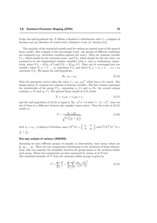
![32 Chapter 3. Statistical Processing of fMRI Data
analysis, proposed in this section, is generic and applicable in all three cases.
3.1.1 Random variables
In our statistical process of fMRI-data, we have to deal with hypothesis tests, probability
distributions, and thus with random variables. To introduce these topics, we shortly
describe the tools which are necessary for their understanding.
A random variable is in our case simply the numerical variable under consideration.
For each trial, a real (discrete) signal x[.] is obtained as a realization of the random
process X[.]. The random variable is represented with a capital letter and its realization
with a lower-case letter. An example of a random process is the game of dice, where the
random variable represents the outcomes of the dice. Since the outcome is stochastic,
only a probability that the random variable X may take a certain value x can be given.
The probability function of X[.] is a function pX (x) which assigns probabilities to all
possible outcomes. That is
pX (x) = P(X = x). (3.1)
A probability function must satisfy the following properties:
(i) pX (x) ≥ 0, for all x ∈ A,
(ii) x∈A pX (x) = 1,
with A the domain of values that X can take. In the continuous case, the random variable
is described by the probability density function pX , defined on the domain A. It satisfies
the following properties:
(i) pX (x) ≥ 0, for all x ∈ A,
(ii) x∈A
pX (x)dx = 1,
(iii) for any interval [a, b] ∈ A,
P(a ≥ X ≥ b) =
b
a
pX (x)dx.
A proposition x ≥ a—like we make it for a hypothesis test—for the random variable
X and a proposition y ≥ b for a random variable Y are independent, if and only if
P(x ≥ a ∧ y ≥ b) = P(x ≥ a)P(y ≥ b) for all a and b. Intuitively, X and Y are
independent if any information about one variable doesn’t tell anything about the other
variable; otherwise
P(x ≥ a ∧ y ≥ b) = P(x ≥ a|y ≥ b)P(y ≥ b). (3.2)](https://image.slidesharecdn.com/0eba55bf-42a7-4963-8f0c-60b852f024ac-160911124222/85/feilner0201-42-320.jpg)
![3.1. Statistical tools 33
In general, we have
P(x ≥ a ∨ y ≥ b) = P(x ≥ a) + P(y ≥ b) − P(x ≥ a ∧ y ≥ b), (3.3)
and when X and Y are mutually exclusive, we obtain P(x ≥ a ∨ y ≥ b) = P(x ≥
a) + P(y ≥ b).
A discrete stochastic process is stationary when the random vectors
(X[0], X[1], . . ., X[n − 1]) and (X[i], X[i + 1], . . . , X[i + n − 1]) have the same
probability density for each n ∈ Z+ and each i ∈ Z. In other words, when the stochastic
process is observed through a (time) window of length n, then the observed statistics
doesn’t depend on the location (i) of the window. All the statistical properties of a
stationary stochastic process are time-independent. One example of a stationary random
variable is an independent and identically distributed (i.i.d.) random variable. For
an i.i.d. process, all random variables X[k], k ∈ Z, have the same probability density
and are independent. Thus an i.i.d. process is statistically fully described by only one
probability distribution for one random variable, for example X[0].
If a discrete random variable X can take values x1, x2, . . . , xn, with probabilities
p1, p2, . . . , pn, then the expected value is defined as
E[X] =
N
i=1
xipi. (3.4)
In the continuous case, we obtain
E[X] =
∞
−∞
xp(x)dx. (3.5)
The variance of X is given for µ = E[X] by
var[X] = E (X − µ)2
(3.6)
= E X2
− (E[X])
2
. (3.7)
A discrete stochastic process X[.] is weakly stationary or wide-sense stationary, when
both E[X[i]] and E[X[i+k]X[i]] for k ∈ Z are independent of i.
In the following section some properties of the expected value are given, for the proof
see [28]:
If X is any random variable then
E[bX + c] = bE[X] + c, (3.8)
when b and c are constants.
If X and Y are any two random variables then
E[X + Y ] = E[X] + E[Y ]. (3.9)](https://image.slidesharecdn.com/0eba55bf-42a7-4963-8f0c-60b852f024ac-160911124222/85/feilner0201-43-320.jpg)
![34 Chapter 3. Statistical Processing of fMRI Data
If X and Y are independent random variables, then
E[XY ] = E[X]E[Y ] (3.10)
and
var[X + Y ] = var[X] + var[Y ]. (3.11)
For any random variable X, it holds that var[cX] = c2
var[X] and var[X + c] = var[X].
A stochastic process X[.] is called white noise with variance σ2
, when X[.] is weakly
stationary, E[X[i]] = 0 and
RX [k] = E[X[i + k]X[i]]
= σ2
δ[k], (3.12)
where RX [.] is the autocorrelation function of X[.].
3.1.2 Multivariate random variables
Suppose we have n p-dimensional observations X[1], X[2], . . . , X[n]. Then each X[i] =
(X1[i], . . . , Xp[i])T
denotes a random vector of dimension p, where p random variables
X1[i], . . . , Xp[i] are defined on a sample space. The mean vector of X, denoted by ¯X, is
given by:
¯X =
1
n
n
i=1
X[i]
=
¯X1
...
¯Xp
. (3.13)
The empirical scatter covariance matrix S of the n p-variate random vectors X[i] is a
p × p matrix
S =
1
n − 1
n
i=1
(X[i] − ¯X)(X[i] − ¯X)T
(3.14)
The expected value of S is the covariance matrix defined by
E[S] =
var[X1] cov[X1, X2] . . . cov[X1, Xp]
cov[X2, X1] var[X2] . . . cov[X2, Xp]
...
...
...
...
cov[Xp, X1] cov[Xp, X2] . . . var[Xp]
. (3.15)](https://image.slidesharecdn.com/0eba55bf-42a7-4963-8f0c-60b852f024ac-160911124222/85/feilner0201-44-320.jpg)
![3.1. Statistical tools 35
Univariate Multivariate
Normal Multivariate normal
Variance Covariance (dispersion) matrix
χ2
-distribution Wishart’s distribution
Student’s t-distribution Hotelling’s T 2
Fisher’s z-distribution Ratio of two covariance-type determinants
Maximum likelihood estimation Maximum likelihood estimation
Analysis of variance (ANOVA) Multivariate analysis of variance (MANOVA)
Table 3.1: Correspondence between univariate and multivariate statistics [78].
The covariance matrix can as well be expressed by:
S = XX
T
− ¯X¯XT
. (3.16)
Table 3.1 provides a brief summary of some results in multivariate theory that are a
generalization of standard notations in the univariate statistical theory [78, 89].
3.1.3 Probability density distributions
We now briefly describe some probability distributions that will be relevant in the context
of fMRI.
z-distribution
Let x be a normally distributed random variable with mean µ and standard deviation σ.
Then, the normalized variable
z =
x − µ
σ
is Gaussian with mean = 0 and standard deviation = 1.
It has a so-called z-distribution (normalized Gaussian), which is given by
F(z) =
1
√
2π
e− 1
2 z2
,
in one dimension. In several dimensions; i.e., x = (x1, ..., xD), we have
F(x) =
1
(2π)
D
2
√
det A
e−
(x−µµµ)T A−1(x−µµµ)
2 , (3.17)
where µ = E[x] and A = E[(x − µ)
T
(x − µ)].](https://image.slidesharecdn.com/0eba55bf-42a7-4963-8f0c-60b852f024ac-160911124222/85/feilner0201-45-320.jpg)
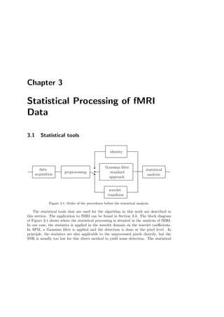
![3.1. Statistical tools 37
0 5 10 15
0
0.05
0.1
0.15
0.2
0.25
ν=3
ν=7
Figure 3.3: Probability density of the χ2
-distribution for several degrees of freedom.
In particular:
√
n − 1
x − E[x]
n
k=1 (xk − x)2
follows a t-distribution with n − 1 degrees of freedom.
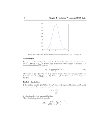
F-distribution
If Y1 and Y2 are independent χ2
-distributed random variables with ν1, ν2 degrees of
freedom, then the random variable
F =
Y1
ν1
Y2
ν2
is F-distributed. The F-distribution is given by
F(t) =
Γ ν1+ν2
2
Γ ν1
2 Γ ν2
2
ν
ν1
2
1 ν
ν2
2
2
t
ν1−2
2
+
(ν1t + ν2)
ν1+ν2
2
.
Hotelling’s T 2
-distribution
If x and M are independently distributed as N(µ, Σ) and Wp(Σ, m), respectively, then
m(x − µ)T
M−1
(x − µ) ∼ T 2
(p, m), (3.19)](https://image.slidesharecdn.com/0eba55bf-42a7-4963-8f0c-60b852f024ac-160911124222/85/feilner0201-47-320.jpg)
![3.2. Hypothesis testing 39
where Wp(Σ, m) is defined as follows:
if M is a matrix of (p×p)-dimension and can be written as M = XT
X, where X is of size
(m × p) and is N(0, Σ) distributed, then M is said to have a Wishart distribution with
scale matrix Σ and degrees of freedom of m. The Wishart distribution is the multivariate
version of the χ2
-distribution (cf. Table 3.1) and is written as M ∼ Wp(Σ, m).
Moreover,
T 2
(p, m) = m
χ2
p
χ2
m−p+1
=
mp
m − p + 1
Fp,m−p+1 (3.20)
(3.21)
For derivations and proofs, see [97].
If ¯x and S are the mean vector and covariance matrix of a sample of size n from
Np(µ, Σ) than
(n − 1)(¯x − µ)T
S−1
(¯x − µ) ∼ T 2
(p, n − 1). (3.22)
Central limit theorem
Let X1, X2, . . . be independent, identically distributed (i.i.d.) random variables with
expected value E[Xi] = µ and variance var[Xi] = σ2
< ∞ for i ∈ N. Then for every
t < ∞, it holds that
lim
n→∞
P
n
i=1(Xi − µ)
σ
√
n
≤ t =
1
√
2π
t
−∞
e− x2
2 dx. (3.23)
This theorem states that the distribution of the sum X1 + X2 + · · · + Xn can be approx-
imated by a normal distribution with expected value E[X1 + · · · + Xn] = nE[Xi] = nµ
and variance var[X1 + · · · + Xn] = nvar[Xi] = nσ2
, when n is large.
3.2 Hypothesis testing
In this section, we describe the validation or rejection of a hypothesis, based on a finite
number of realizations of some random variables. We consider data that can be described
by a probability distribution. In particular, one of its statistical parameter µ is unknown.
We propose a particular value µ0 for µ and we want to be able to decide from a set of
measurements whether the hypothesis µ = µ0 is trustworthy or must be rejected. A
numerical method for testing such a hypothesis or theory is called hypothesis test or sig-
nificance test. In any such situation, the experimenter has to decide, if possible, between
two rival possibilities. The hypothesis we want to test is called the null hypothesis, and is](https://image.slidesharecdn.com/0eba55bf-42a7-4963-8f0c-60b852f024ac-160911124222/85/feilner0201-49-320.jpg)
![40 Chapter 3. Statistical Processing of fMRI Data
denoted by H0. Any other hypothesis is called the alternative hypothesis, and is denoted
by H1. Thus, such a hypothesis test could be:
1. Null hypothesis H0: µ = µ0,
2. Alternative hypothesis H1: µ > µ0.
The standard procedure is to summarize the data by a test statistic y that depends on
the value µ0. Under the null hypothesis, the distribution for this statistic is known. Even
when H0 is true, we cannot expect that µ matches µ0 exactly. Thus we have to think of
an expected bound, which should not be exceeded. If y exceeds this expected bound, the
null hypothesis is rejected and the alternative hypothesis H1 is accepted; the decision
is made by setting a threshold. Thus, with such a hypothesis test, we can never state
that H0 is true, only that it is trustworthy. On the other hand, we can state that H0 is
wrong, with high evidence whenever we reject the null hypothesis.
Given some probability value α, we compute the threshold t such that the probability
that y exceeds t is equal to α, assuming that H0 is true:
P(y ≥ t) = α.
In other words, α is the probability of observing higher values than t by chance, given
that the null hypothesis is true. This probability α is called the level of significance of
the test.
The p-value is the probability that a test statistic is at least as extreme as the one
observed, given that the null hypothesis is true. The smaller the p-value, the stronger
the evidence against H0. If the level of significance of the test statistic is less than 5 %,
we say that the result is significant at the 5 % level. This is generally considered as a
reasonable evidence that H0 is not true.
The test on the set of data has to be adapted to its distribution, which transforms the
values into p-values.
3.2.1 Two-tailed test
In the section above, the alternative hypothesis to H0 is defined as H1: µ > µ0. Any
such test where the alternative hypothesis tests for values only higher than µ0 or only
lower than µ0, the test is called one-tailed or one-sided. But H1 can also be defined as
H1: µ = µ0, where the departure of the null hypothesis in both directions is of interest.
This means that we are interested in significantly high or low results, which is called
appropriately a two-tailed test [28].
3.2.2 z-test
Here, a random sample with size n is taken from a normal distribution with unknown
mean µ (cf. Section 3.1.3). We want to test if the sample mean is equal to a particular](https://image.slidesharecdn.com/0eba55bf-42a7-4963-8f0c-60b852f024ac-160911124222/85/feilner0201-50-320.jpg)
![3.2. Hypothesis testing 41
value µ0 or not. Thus the null hypothesis is given by
H0 : µ = µ0. (3.24)
If the variance σ2
is constant over the whole set of samples and is known, then ¯x =
1
n
n
i=1 xi follows a normal-distribution, and a z-test may be applied:
y =
¯x − µ0
σ√
n
. (3.25)
If a two-tailed test is appropriate, the level of significance is obtained by calculating the
threshold t such that
α = P(|y| ≥ |t|) (3.26)
= 2P(y ≥ |t|); (3.27)
i.e., t is the p-value, related to the significance level α.
3.2.3 Student’s t-test
If the variance σ2
is unknown, we apply a t-test (see Student’s t-distribution in Section
3.1.3) with n−1 degrees of freedom. The corresponding test statistic with ¯x = 1
n
n
i=1 xi
is
y =
¯x − µ0
s√
n
(3.28)
where µ0 = E[¯x] and where
s2
=
1
n − 1
n
i=1
|xi − ¯x|2
. (3.29)
Two sample t-test
The t-test described above is a one sample t-test. In the case of a two sample t-test, the
means of two samples of data are compared. The sizes of the two samples are n1 and n2,
respectively, with unknown statistical means µ1 and µ2, respectively and same standard
deviation σ. The first sample mean (measured mean) will be denoted by ¯x1 and the
second one will be denoted by ¯x2. The problem now is to test the null hypothesis
H0 : µ1 = µ2. (3.30)
The alternative hypothesis is expressed in the case of a two-tailed test by
H1 : µ1 = µ2. (3.31)](https://image.slidesharecdn.com/0eba55bf-42a7-4963-8f0c-60b852f024ac-160911124222/85/feilner0201-51-320.jpg)
![42 Chapter 3. Statistical Processing of fMRI Data
The test statistic is, according to (3.28), obtained by
t =
¯x1 − ¯x2
s 1
n1
+ 1
n2
. (3.32)
The unbiased estimate s2
of σ2
is given by
s2
=
(n1 − 1)s2
1 + (n2 − 1)s2
2
n1 + n2 − 2
, (3.33)
where the standard deviation s1 is obtained by
s2
1 =
n1
i=1
(x1[i] − ¯x1)2
n1 − 1
(3.34)
and the standard deviation s2 is given by
s2
2 =
n2
i=1
(x2[i] − ¯x2)2
n2 − 1
. (3.35)
Note, that in the case where n1 = n2, the estimate of σ2
is given by
s2
=
s2
1 + s2
2
2
. (3.36)
The paired t-test
This test is applied when the experiments are carried out in pairs. Here, the difference
between each pair is of interest.
Let us assume we have n pairs x1[i] and x2[i] for i = 1, . . . , n, which are independent
observations of populations with means µ1 and µ2. Then the null hypothesis is described
as
H0 = µ1i = µ2i for all i = 1, . . . , n. (3.37)
The difference of the pairs is given by
di = x1[i] − x2[i] i = 1, . . . , n, (3.38)
where di is a sample of size n with mean zero. The average difference is denoted by
¯d =
n
i=1 di and the standard deviation is denoted by s. Then the test statistic is given
by
y =
¯d
s√
n
, (3.39)
where the standard deviation is obtained according to (3.29).](https://image.slidesharecdn.com/0eba55bf-42a7-4963-8f0c-60b852f024ac-160911124222/85/feilner0201-52-320.jpg)
![44 Chapter 3. Statistical Processing of fMRI Data
follows an F-distribution with p and (n − p) degrees of freedom (p degrees of freedom in
the numerator and n − p degrees of freedom in the denominator) [7, 60].
3.2.6 Multiple testing
We have different possibilities to set the threshold t for the hypothesis test. Some of
them are discussed below.
Bonferroni-correction
The above reasoning of setting the threshold does not apply anymore if we look at several
test statistics jointly. In the case of 5 % of the test statistics, H0 would be rejected by
error, when no multiple correction is applied. Thus we have to correct for multiple testing.
Since we don’t want to have more than α% of wrong rejections of H0 globally, we have
to divide α by the number of test statistics. This is known as Bonferroni-correction [21]
for multiple testing:
α =
α
N
, (3.44)
where N = number of test statistics.
It is almost exact, when no correlation is present, otherwise still correct but perhaps
too conservative. It is exact (and not only almost exact) with (1 − α )N
= 1 − α, i.e.,
α = 1 − (1 − α)N α
N (cf. Paragraph “Probability of the maximum”). Bonferroni’s
correction is the most conservative (=safe) approach to deal with multiple tests.
Binomial law
Another possibility for multiple correction is to determine the number of false rejections
of H0 (n0) that is expected from our significance level α. The probability to observe n0
false rejections in a random field with noise only follows a binomial distribution:
P(n = n0) =
N
n0
pn0
(1 − p)N−n0
, (3.45)
with p = P(y > t) and N = number of test statistics. Equation (3.45) holds when
no correlation between the test statistics is present. Since we know how many wrong
rejections we should expect, we are able to compare them with the effectively observed
ones. If there are significantly more than expected, then we have a significant result
within the samples of test statistics. Yet, we have not localized it, because this is a
global test only.
In the case of Bonferroni-correction, n0 = 0 and the mean value E[n] of appearance of a
false rejections is equal to Np = α (usually α = 0.05). Consequently the approach is](https://image.slidesharecdn.com/0eba55bf-42a7-4963-8f0c-60b852f024ac-160911124222/85/feilner0201-54-320.jpg)
![46 Chapter 3. Statistical Processing of fMRI Data
The next step is to calculate the expected Euler characteristic E[χt] of the statistical
parameter map. E[χt] is used to approximate the probability that the maximum value
on the map (zmax), when no activation is present, is greater than a given threshold t
under the null hypothesis H0. χt is a geometrical measure that counts the number of
isolated regions on a volume map after thresholding with t, provided the excursion set
contains no holes and doesn’t touch the boundary of the search volume (approximation
for a rather high t) [2, 3, 156]. For such a t, it holds that
P(zmax ≥ t) ≈ P(χt ≥ 1) ≈ 1 − eE[χt]
≈ E[χt]. (3.48)
Moreover the clusters over such a high threshold t are independent and their number Ct
follows approximately a Poisson distribution with mean E[χt]:
P(Ct = x) =
1
x!
(E[χt])x
e−E[χt]
= Υ(x, E[χt]). (3.49)
0 0.5 1 1.5 2 2.5 3 3.5 4 4.5 5
0
5
10
15
20
25
30
Z score threshold
ExpectedECforthresholdedimage
Figure 3.6: Expected Euler characteristic for smoothed image with 256 RESELS, corresponding
to equation (3.50).
The expected Euler characteristic is given by:
E[χt] = λ(V ) |Λ|(2π)− D+1
2 HeD (t)e− t2
2 , (3.50)
where λ(V ) represents the volume and HeD (t) is the Hermite polynomial of degree D in
t. t represents here the value to test, the local maximum of a potential activation. |Λ|
is a smoothness factor which allows to obtain an estimation of the smoothness in the
volume, where Λ represents the variance covariance matrix tested in D dimensions. It is
shown that ([156])
λ(V ) |Λ| = RESELS(4 loge 2)
D
2 . (3.51)](https://image.slidesharecdn.com/0eba55bf-42a7-4963-8f0c-60b852f024ac-160911124222/85/feilner0201-56-320.jpg)
![3.3. fMRI applications 47
For a volume, (3.50) becomes:
E[χt] = λ(V ) |Λ|(2π)−2
(4t2
− 2)e− t2
2 . (3.52)
Several assumptions have to be made for equations (3.48) and (3.50) to hold: the
threshold t must be sufficiently high, the volume V must be large compared to resolution
elements in the map, and finally the discrete statistical parameter map must approxi-
mate a continuous zero-mean univariate homogeneous smoothed Gaussian Random Field
(GRF). In other words, the autocorrelation function of the field must be a Gaussian. An-
other assumption is the spatial stationarity which, in our view, is a wrong assumption.
These assumptions are discussed more exhaustively in [111].
In addition to testing for the intensity of an activation, SPM also tests for the sig-
nificance of its spatial extent, and for the significance of a set of regions. For the corre-
sponding theory, we refer to [111].
SPM99 takes care of two aspects which can be formulated more precisely and are de-
scribed in [157]. The first improvement concerns the Euler characteristics, which depends
not only on the number of RESELS anymore, but also on the shape of the volume. This
precision is especially effective when the volume in which the RESELS are contained is
small. In contrast, when the volume is large, the two approaches give similar results.
The second improvement concerns the degrees of freedom. In the case of few degrees of
freedom, the SPM scores, which are based on z-statistics, are not adequate anymore using
the random field theory. Thus the new approach generates thresholds for the t-statistics,
from which the z-scores are derived [69, 155, 63].
3.3 fMRI applications
In this section, we briefly discuss fMRI noise and then describe the statistical procedure
of our fMRI analysis algorithm.
3.3.1 Noise in fMRI data
Since fMRI-data are extremely noisy, we devote a section to the analysis and modelling
of this particular noise.
Origin
The noise in fMRI data originates from several sources. There is the noise of the mea-
surement instrument (e.g., the scanner), in particular, due to hardware imperfections
[94], but there is also noise arising from the patient’s body, which is the main source of
disturbance in an image [51]. Some of the main sources are:](https://image.slidesharecdn.com/0eba55bf-42a7-4963-8f0c-60b852f024ac-160911124222/85/feilner0201-57-320.jpg)
![48 Chapter 3. Statistical Processing of fMRI Data
Thermal noise. The most dominant source of thermal noise is the one arising from the
patient in the scanner. Thermal vibrations from ions and electrons induce noise
in the receiver coil. Since the noise level depends on how many ions and electrons
are contributing to the signal, it is important to adjust the size of the receiver
coil to the object which is imaged. For this reason, MRI has different coils for
different regions of interest, like the head or the spine. The disadvantage is that
some small coils have an image intensity which is non-uniform over the region of
interest. Other sources of thermal noise are quantization noise in the A/D devices,
preamplifier/electronic noise, and finally thermal noise in the RF coils [106, 24].
Motion of the subject. Even when fixing the head of the patient during acquisition,
head motion cannot be completely avoided. Such head motions can arise, for exam-
ple, from respiration. Task-correlated head movements are especially disturbing,
since these movement effects can look like task activation. Motion of the order of
1
10 voxel may produce 1−2% signal changes, which is not negligible. In comparison,
fMRI BOLD effects are very small: 1 − 5% signal changes with a magnetic field of
1.5 T [37, 25]. This calls for the use of accurate image registration algorithms in a
preprocessing stage (cf. Section 2.6).
Noise due to physiological activities. The cardiac cycle causes vessel pulsations,
cerebrospinal fluid movements, and tissue deformations, which all produce fMRI
signal variations [39]. The approaches to mitigate cardiac effects are to record the
cardiac cycle, to estimate its influence on the fMRI signal a posteriori, and to fi-
nally remove it.
Respiratory variations also induce signal changes in the head. Respiration causes
blood pressure changes that may result in slight modifications of the size of the
CSF and venous blood spaces in the brain. A special possible respiration effect for
some subjects is the unconsciously gating of their breathing to the task, especially
when this task is very regular. A subject may hold off breathing until his response
to a trial [106, 109, 18].
Low frequency drift. Low frequency drifts (0.0-0.015 Hz) and trends are often re-
ported in fMRI data. It is one of the most poorly understood source of signal
variations. Investigations by Smith et al. [130] suggest that scanner instabilities
and not motion or physiological noise may be the major cause of the drift.
Spontaneous neural and vascular fluctuations and behavior variations. There
are a variety of neuro- and vascular physiological processes that lead to fluctuations
in the BOLD signal intensity. In addition to this background processes, there are
also variations in the way in which subjects perform tasks from trial to trial [106].
Artifacts in Rapid Imaging Methods. The main disadvantages and artifacts of
rapid imaging methods are [106]:](https://image.slidesharecdn.com/0eba55bf-42a7-4963-8f0c-60b852f024ac-160911124222/85/feilner0201-58-320.jpg)
![3.3. fMRI applications 49
Limited spatial resolution.
Ghosting (affects mostly EPI) [30, 123, 32].
Susceptibility distortions: differences in magnetic susceptibilities between air
and watery tissue in the head result in non-uniformities in the magnetic fields,
which causes artifacts. In the EPI technique, these artifacts result mainly in
geometric distortions [84]. The distortions can be a shift, shear, stretch, or
squish of the object; in most cases these effects are local. Fat is an example
that can cause artifacts like shifting and therefore rapid imaging techniques
use “fat suppression”. All the fMRI-data used in this work were acquired
under fat suppression.
Characterization
To get a better understanding of the statistical nature of our data, we try to determine
the main properties of the noise. This step is crucial since we are aiming at an accurate
and rigorous statistical analysis of the results of fMRI experiments.
We make the general hypothesis that the noise follows a Gaussian distribution. This
assumption is certainly reasonable when working with averaged finite energy data (due
to the central limit theorem, cf. Section 3.1.3), as is the case here. The key question to
be answered concerns the covariance structure of the noise (independence, stationarity
over space and time).
Time variance over space. We question whether the variance is homogeneously dis-
tributed over space, or whether the variance differs significantly within the volume. The
hypothesis for the following calculation is that the time sequence of each voxel is inde-
pendent and normally distributed with variance σ; then, defining s2
k =
n
τ=1
(xk(τ)−xk)2
n−1
with xk = 1
n
n
τ=1 xk(τ), we know that
s2
k
σ2 follows a χ2
distribution with n − 1 degrees
of freedom (see Section 3.1.3), where k is a 3D integer index locating the voxel in the
volume.
Therefore, we may write a confidence interval for this estimate as
P(a ≤ (n − 1)
s2
k
σ2
ξ
≤ b) = α, (3.53)
where P is the χ2
cumulative probability, see Section 3.1.3; this means, that (n − 1)
s2
k
σ2
will fall within the interval [a, b] with probability α.
“a” and “b” are to be computed in such a way as to obtain the smallest interval, depending
on the confidence interval probability α. Let us denote by a(α) and b(α) those optimal](https://image.slidesharecdn.com/0eba55bf-42a7-4963-8f0c-60b852f024ac-160911124222/85/feilner0201-59-320.jpg)
![50 Chapter 3. Statistical Processing of fMRI Data
values. Then we get an interval for σ2
:
(n − 1)
s2
k
b(α)
≤ σ2
≤ (n − 1)
s2
k
a(α)
. (3.54)
To get the smallest interval for σ2
, we minimize 1
a − 1
b under the condition of P(a ≤
ξ ≤ b) = α. Using Lagrange multipliers, we define the auxiliary function
f(a, b, λ) =
1
a
−
1
b
− λP(a ≤ ξ ≤ b). (3.55)
Taking the partial derivatives, we get
∂f(a, b, λ)
∂a
= −
1
a2
+ λp(a)=0 (3.56)
∂f(a, b, λ)
∂b
=
1
b2
− λp(b) =0, (3.57)
since P(a ≤ ξ ≤ b) =
b
a p(ξ)dξ. From equation (3.56) and (3.57), we obtain the
optimality condition:
a2
p(a) = b2
p(b). (3.58)
Below is the code that determines the smallest interval by an iterative process which
converges to a solution where (3.53) and (3.58) are satisfied.
N := degree of freedom;
a(1) := 0;
for i := 1 to 100 step 1 do
b(i) = chi2inv(α + chi2cdf (a(i), N), N);
a(i + 1) = a(i) + 0.1 ∗ (b(i)2
∗ chi2pdf (b(i), N) − a(i)2
∗ chi2pdf (a(i), N));
end,
We observe that, on a logarithmic scale, the intervals have a constant size
log(σ2
) − log(s2
k) ∈ [min, max]
∆
, (3.59)
where
min = log
n − 1
b(α)
,
max = log
n − 1
a(α)
,](https://image.slidesharecdn.com/0eba55bf-42a7-4963-8f0c-60b852f024ac-160911124222/85/feilner0201-60-320.jpg)
![3.3. fMRI applications 51
× ×
log(s2
k) log(s2
k )
∆
Figure 3.7: Equidistant confidence intervals on logarithmic scale. s2
k and s2
k are significantly
different.
which suggests a natural quantization step for the representation of the variance data
s2
k. Since we look at the whole image, the value α is corrected for multiple testing with
the Bonferroni method.
We thus obtain for each log(s2
k) an uncertainty interval ∆, wherein the true log(σ2
)
lies with the probability α (chosen to be close to 1). If two intervals are not adjacent,
then we can assert that the corresponding estimates for σ2
are significantly different.
Applying this to one slice of different data-set, we get the result as depicted in Fig-
ure 3.8. From experiments such as these, we conclude that the variance is generally not
constant over space, contrary to what has often been stated in the literature [120, 52].
The variances, however, appear to be strongly correlated over space—in other words,
their variation is usually small within the neighborhood of a pixel.
Stationarity and time-independence. We take the time sequence of the rest state (B)
for each voxel and compute the variances of the first and second half of the time sequence.
Then, applying an F-test (see Section 3.2.4), we can check if the variances differ signifi-
cantly, in which case at least one of our hypotheses (stationarity or time-independence)
will fail:
ρk =
n
2 −1
τ=0 (xk(τ) − ξ0)2
n
2 −1
τ=0 (xk(τ + n
2 ) − ξ1)2
(3.60)
where
ξ0 =
1
n
2
n
2 −1
τ=0
xk(τ)
ξ1 =
1
n
2
n
2 −1
τ=0
xk(τ +
n
2
).
We note that most statistical methods developed so far in the fMRI literature make the
assumption of stationarity and time-independence.
We applied this test to several of our data sets. Most of the slices show no detection.
However, in some cases the number of detections exceeds the false detection rate of the](https://image.slidesharecdn.com/0eba55bf-42a7-4963-8f0c-60b852f024ac-160911124222/85/feilner0201-61-320.jpg)
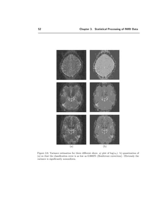
![3.3. fMRI applications 53
Figure 3.9: Slices of one data set which show some detections. The threshold of the test is
Bonferroni-corrected. We believe the false detections arose mostly from motion artifacts.
Bonferroni-correction. Those detected pixels are mostly on the border of the brain or
around the eyes. Thus we have some indications that the cases of false detections are
due to motion artifacts which could not be prevented by the realignment procedure (cf.
Figure 3.9).
3.3.2 Deterministic model
In order to make a statistical inference, we first need to specify a model. Three possible
data models at pixel k are being considered, from the simplest to the more complex.
Gaussian white noise assumption
Model 1: In some studies, the noise has been assumed to be white Gaussian [120, 52].
The corresponding model is
xk(τ) = µk(τ) + ek(τ) · σ,](https://image.slidesharecdn.com/0eba55bf-42a7-4963-8f0c-60b852f024ac-160911124222/85/feilner0201-63-320.jpg)
![54 Chapter 3. Statistical Processing of fMRI Data
where µk is the average hemodynamic function, ek is an i.i.d. normalized noise (E[ek] =
0, E[e2
k] = 1).
The hypothesis is that µk = µ1 during A and µk = µ2 during B. Thus, the detection of
activation uses a statistical test applied on a pixel by pixel basis to determine whether
or not µ1 and µ2 are different.
The white noise hypothesis has the advantage of simplicity. However, we found it to be
inappropriate for our data (cf. Section 3.3.1).
Time-independent, but space-non-stationary white noise
Model 2: In the second model, we assume to have whiteness (over time), but space-varying
(non stationary) Gaussian noise:
xk(τ) = µk(τ) + ek(τ) · σk,
where the variance σk varies over the pixels, but changes only slightly, see Section 3.3.1.
We use this model which is consistent with our finding in Section 3.3.1.
General linear model
Model 3: In the third model we include components that also vary over time (hemody-
namic function or periodic disturbances). They are represented as a weighted sum of c
different functions:
xk(τ) =
c
i=1
αk,igi(τ) + σkek(τ),
where gk(τ) is the explanatory variable and represents an activation function. This
approach offers no extension on the noise description. But its deterministic model offers
the possibility of refinements, e.g., including baseline drifts. The General Linear Model
(GLM) is used among others by SPM, see also Section 2.8.2.
3.3.3 Hypothesis testing for activation
In the case of our algorithm, the sample of the data set to test is the time sequence of
a voxel and we want to decide whether this voxel is activated or not. This procedure is
repeated for all voxels at locations k = (i, j, l) in the volume. To simplify matters, we
will describe the two-dimensional case, where we consider all the pixels k = (i, j) in a
slice. The derivation of the samples to test is as follows: spatial noise is reduced either by
filtering or wavelet transformation in which case the testing is performed in the wavelet
domain. To find the activation, we calculate the pairwise difference between activation
and rest states yielding the sequence difference images xDτ (i, j) = xAτ (i, j) − xBτ (i, j),
where the symbol A stands for the activation state and the symbol B for the rest state.](https://image.slidesharecdn.com/0eba55bf-42a7-4963-8f0c-60b852f024ac-160911124222/85/feilner0201-64-320.jpg)
![3.3. fMRI applications 55
¡ ¡ ¡ ¡ ¡ ¡ ¡ ¡ ¡ ¡ ¡ ¡ ¡ ¡ ¡ ¡ ¡ ¡ ¡ ¡ ¡ ¡ ¡ ¡ ¡ ¡ ¡ ¡ ¡ ¡ ¡ ¡ ¡ ¡ ¡ ¡ ¡ ¡ ¡ ¡ ¡ ¡ ¡ ¡ ¡ ¡ ¡ ¡ ¡ ¡ ¡ ¡ ¡ ¡ ¡ ¡ ¡ ¡ ¡ ¡ ¡ ¡ ¡ ¡ ¡ ¡ ¡ ¡ ¡ ¡ ¡ ¡ ¡ ¡ ¡ ¡ ¡ ¡ ¡ ¡
¢¡¢¡¢¡¢¡¢¡¢¡¢¡¢¡¢¢¡¢¡¢¡¢¡¢¡¢¡¢¡¢¡¢¢¡¢¡¢¡¢¡¢¡¢¡¢¡¢¡¢¢¡¢¡¢¡¢¡¢¡¢¡¢¡¢¡¢¢¡¢¡¢¡¢¡¢¡¢¡¢¡¢¡¢¢¡¢¡¢¡¢¡¢¡¢¡¢¡¢¡¢¢¡¢¡¢¡¢¡¢¡¢¡¢¡¢¡¢¢¡¢¡¢¡¢¡¢¡¢¡¢¡¢¡¢¢¡¢¡¢¡¢¡¢¡¢¡¢¡¢¡¢¢¡¢¡¢¡¢¡¢¡¢¡¢¡¢¡¢
£¡£¡£¡£¡£¡£¡£¡£¡££¡£¡£¡£¡£¡£¡£¡£¡££¡£¡£¡£¡£¡£¡£¡£¡££¡£¡£¡£¡£¡£¡£¡£¡££¡£¡£¡£¡£¡£¡£¡£¡££¡£¡£¡£¡£¡£¡£¡£¡££¡£¡£¡£¡£¡£¡£¡£¡££¡£¡£¡£¡£¡£¡£¡£¡££¡£¡£¡£¡£¡£¡£¡£¡££¡£¡£¡£¡£¡£¡£¡£¡£
¤¡¤¡¤¡¤¡¤¡¤¡¤¡¤¡¤¤¡¤¡¤¡¤¡¤¡¤¡¤¡¤¡¤¤¡¤¡¤¡¤¡¤¡¤¡¤¡¤¡¤¤¡¤¡¤¡¤¡¤¡¤¡¤¡¤¡¤¤¡¤¡¤¡¤¡¤¡¤¡¤¡¤¡¤¤¡¤¡¤¡¤¡¤¡¤¡¤¡¤¡¤¤¡¤¡¤¡¤¡¤¡¤¡¤¡¤¡¤¤¡¤¡¤¡¤¡¤¡¤¡¤¡¤¡¤¤¡¤¡¤¡¤¡¤¡¤¡¤¡¤¡¤¤¡¤¡¤¡¤¡¤¡¤¡¤¡¤¡¤
0 1 2 3 4-1-2-3-4
0.1
0.3
0.4
0.2
α
Student’s t-distribution
t
activation
significantno significant
activation
Student’s t-distribution
area=α
2
Figure 3.10: Definition of significance level for the two-tailed t-test.
To decide which pixel is activated, we denote the null hypothesis —the pixel under
consideration is not activated—by H0. Under this hypothesis, µ0 = E[¯xD(i, j)] = 0 and
the distribution for the mean value of each pixel relative to its standard deviation is
known. The corresponding test statistic y(i, j) on the distribution has to be adapted to
the set of data, which transforms the pixel values into p-values. Which test statistic y is
implemented for fMRI data is discussed later in Section 3.3.5. If a test statistic exceeds
some expected bound for ¯xD(i, j), the null hypothesis is rejected and the alternative
hypothesis H1 is accepted: we conclude that the pixel (or, eventually, wavelet coefficient)
is activated:
1. Null hypothesis H0: E[¯xD(i, j)] = 0 (no activation).
2. Alternative hypothesis H1: E[¯xD(i, j)] = 0 translates to |¯xD(i, j)| ≥ t, where t is
our significance threshold as explained in Section 3.2.6.
Given the level of significance (see Section 3.2) α = 0.05, we compute the threshold t
such that the probability that |y(i, j)| exceeds t is less than or equal to α, assuming that
H0 is true.
P(|y(i, j)| ≥ t) = α.
In the hypothesis test of our algorithm, the alternative hypothesis H1 is defined as
E[¯xD(i, j)] = 0, as we saw above. Thus we perform a two-tailed test (see Section 3.2.1).
A two-tailed test is chosen, since in the wavelet domain, the high-pass includes possible
significant high and low coefficients, which are of interest. The low-pass is tested with](https://image.slidesharecdn.com/0eba55bf-42a7-4963-8f0c-60b852f024ac-160911124222/85/feilner0201-65-320.jpg)
![56 Chapter 3. Statistical Processing of fMRI Data
a two-tailed hypothesis test as well. Here, when a significantly low-pass coefficient is
detected, one can think of the negative activation, also called deactivation, such as a
relative decrease of oxyhemoglobin; A deactivation can happen for two reasons: it may
reflect decrease of synaptic activity during the task of interest, or it may reflect an active
increase during the rest task [86].
3.3.4 z-test
If the variance σ2
is constant over the whole set of samples in the image and is known,
then E[¯xD(i, j)] follows a normal-distribution, and a z-test (Section 3.2.2) may be applied
as in [120]:
z(i, j) =
¯xD(i, j) − µ0
σ√
n
. (3.61)
Here a two-tailed test is appropriate too.
3.3.5 Student’s t-test
If the variance σ2
changes with (i, j), as was found to be the case with fMRI data in
Section 3.3.1, we apply a t-test (see Section 3.2.3) with n − 1 degrees of freedom. The
corresponding test statistic is
t(i, j) =
¯xD(i, j) − µ0
sD(i,j)
√
n
, (3.62)
where ¯xD(i, j) = 1
n
n
τ=1 xDτ (i, j) and where
s2
D(i, j) =
1
n − 1 τ
|xDτ (i, j) − ¯xD(i, j)|2
. (3.63)
In our case, µ0 = E[¯xD(i, j)]. The t-test described above is a one sample t-test, since
we compute the difference of the two samples before testing. In the following section, a
method is described, where the number of the samples of the activation state and the
rest state are not the same. Also with SPM (see Section 2.8) one can choose between one
sample t-test, two sample t-test and paired t-test under the category of “basic models”.
Two sample t-test
This case is applied when the number of samples in the activation state and in the rest
state are not the same; in other words, when we cannot make the difference between
these two states before testing. The two samples size will be denoted by nA and nB,](https://image.slidesharecdn.com/0eba55bf-42a7-4963-8f0c-60b852f024ac-160911124222/85/feilner0201-66-320.jpg)
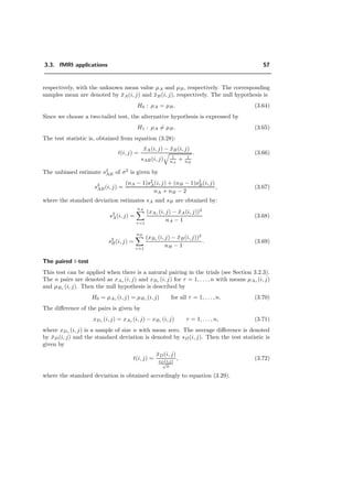
![58 Chapter 3. Statistical Processing of fMRI Data
3.3.6 F-test
Instead of applying a two-tailed t-test to our data, we could also compare the different
estimates of ¯x2
A and ¯x2
B and apply an F-test (see Section 3.2.4).
3.3.7 Hotelling’s T2
-test
As reported in Section 3.2.5, the Hotelling’s T 2
-test is the multivariate version of the
univariate Student’s t-test. In our case, the complex wavelets (see Section 4.4) make the
statistics bivariate. Like in the univariate case, to find the activation, we calculate the
difference between activation and rest states pairwise to produce the sequence difference
images xDτ (i, j) = xAτ (i, j) − xBτ (i, j), where xAτ (i, j) and xBτ (i, j) ∈ C. Thus, we
have to deal with bivariate random vectors (p = 2) X[1], . . . , X[τ], . . . , X[n], where one
dimension of the random vectors represents the real part of the wavelet coefficients, while
the second dimension represents the imaginary part.
The variables x[1], . . . , x[τ], . . . , x[n] represent the samples from one wavelet location
with the mean vector µ = (µ1, µ2)T
. Then we want to test the hypothesis
H0 : µ = µ0, (3.73)
where the hypothetical mean vector µ0 equals in our case to (0, 0)T
. The sample mean
vector and the sample covariance matrix are denoted by ¯xD(i, j) and SD(i, j), respec-
tively. The corresponding test statistic with ¯xD(i, j) = 1
n
n
τ=1 xD(i, j)[τ] is:
T2
(i, j) = n¯xT
D(i, j)S−1
D (i, j)¯xD(i, j), (3.74)
where
SD =
s11 s12
s21 s22
, (3.75)
with
s11 =
1
n − 1
n
τ=1
(x1(i, j)[τ] − ¯x1(i, j))
2
s22 =
1
n − 1
n
τ=1
(x2(i, j)[τ] − ¯x2(i, j))2
s12 =
1
n − 1
n
τ=1
(x1(i, j)[τ] − ¯x1(i, j)) (x2(i, j)[τ] − ¯x2(i, j))
s21 = s12.](https://image.slidesharecdn.com/0eba55bf-42a7-4963-8f0c-60b852f024ac-160911124222/85/feilner0201-68-320.jpg)
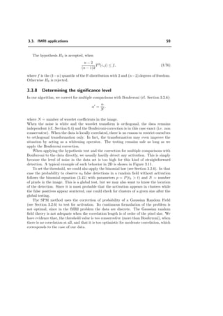
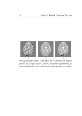
![62 Chapter 4. Wavelets
where Wj is called the detail space (there are several choices for Wj , one of them being
the ⊥ complement of Vj). Iterating equation (4.2) gives
Vj+1 = ⊕j
k=−∞Wk. (4.3)
The second requirement for an MRA is that all functions in L2
(R) are included at the
finest resolution and only the zero function at the coarsest level. Hence, due to (4.1), we
have limj→−∞ Vj = {0} and limj→∞ Vj → L2
(R). Hence, letting j → +∞ gives
L2
(R) = ⊕∞
k=−∞Wk. (4.4)
The last requirement for an MRA is that there exist a function φ such that {φ(t−k)}k∈Z
forms a Riesz basis for V0.
To summarize, a multiresolution analysis of L2
(R) is a nested sequence of subspaces
{Vj}j∈Z such that
i) · · · ⊂ V−1 ⊂ V0 ⊂ V1 ⊂ · · · ⊂ L2
(R) (4.5)
ii)
j
Vj = {0},
j
Vj = L2
(R) (4.6)
iii) f(t) ∈ Vj ⇐⇒ f(2t) ∈ Vj+1 (4.7)
iv) There exists a function φ(t), called the scaling function,
such that {φ(t − k)} is a Riesz basis of V0. (4.8)
Consequently: f(t) ∈ V0 =⇒ f(t − k) ∈ V0
φ(t) is defined to be a valid scaling function of L2 if and only if:
i) A ≤ k∈Z
ˆφ(ω + 2πk)
2
≤ B (Riesz basis) (4.9)
ii) φ(t) =
√
2 k h[k]φ(2t − k) (two-scale relation) (4.10)
iii) k∈Z φ(t − k) = 1 (partition of unity) (4.11)
Under slight constraints, these three conditions are equivalent to the four conditions
which define an MRA.
(4.11) implies that
∞
−∞ φ(t)dt = 1. Thus with the two scale relation (4.10) we obtain
k
h[k] =
√
2. (4.12)
If φ is orthonormal, then
k
|h[k]|2
= 1 and
k
h[k]h∗
[k + 2l] = 0, l = 0. (4.13)](https://image.slidesharecdn.com/0eba55bf-42a7-4963-8f0c-60b852f024ac-160911124222/85/feilner0201-72-320.jpg)
![4.1. Introduction 63
The detail space W0 has also a Riesz basis {ψ(t − k)}k∈Z, called the wavelet basis. The
function ψ(t) is referred to as the mother wavelet. Since W0 ⊂ V1, ψ(t) can be written
as a superposition of the basis functions for V1:
ψ(t) =
√
2
k
g[k]φ(2t − k), (4.14)
which is called the wavelet equation. From the requirement that
∞
−∞
ψ(t)dt = 0, we
obtain
k
g[k] = 0. (4.15)
All these relations can be expressed in the Fourier domain. With ˆφ(ω) =
∞
−∞
φ(t)e−jωt
dt and H(ω) = 1√
2 k h[k]e−jkω
and correspondingly ˆψ(ω) =
∞
−∞ ψ(t)e−jωt
dt and G(ω) = 1√
2 k g[k]e−jkω
, we obtain
ˆφ(ω) = H
ω
2
ˆφ
ω
2
(4.16)
ˆψ(ω) = G
ω
2
ˆφ
ω
2
. (4.17)
The orthogonality conditions can also be expressed in the frequency domain. It is equiv-
alent to claim that {φ(t − k)} is orthonormal and to have:
∞
l=−∞
|ˆφ(ω + 2πl)|2
= 1. (4.18)
To orthogonalize a basis function which is not orthogonal, we divide its Fourier transform
by the square root of the left hand side of (4.18):
ˆφortho(ω) =
ˆφ(ω)
∞
l=−∞ |ˆφ(ω + 2πl)|2
. (4.19)
It can be verified that for φ to be orthogonal, it is necessary and sufficient that
|H(ω)|2
+ |H(ω + π)|2
= 1. (4.20)
This relation is derived simply by inserting (4.16) into (4.18). Similarly, {ψ(t − k)} is
orthonormal if
∞
l=−∞
| ˆψ(ω + 2πl)|2
= 1 (4.21)](https://image.slidesharecdn.com/0eba55bf-42a7-4963-8f0c-60b852f024ac-160911124222/85/feilner0201-73-320.jpg)
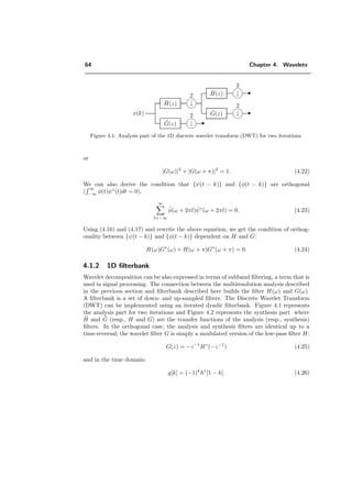
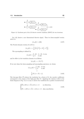
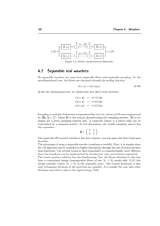
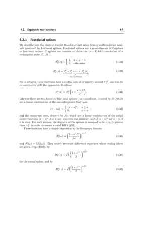
![2
↓ •
Figure 4.1: Analysis part of the 1D discrete wavelet transform (DWT) for two iterations.
or
|G(ω)|2
+ |G(ω + π)|2
= 1. (4.22)
We can also derive the condition that {ψ(t − k)} and {φ(t − k)} are orthogonal
(
∞
−∞ φ(t)ψ∗
(t)dt = 0),
∞
l=−∞
ˆφ(ω + 2πl) ˆψ∗
(ω + 2πl) = 0. (4.23)
Using (4.16) and (4.17) and rewrite the above equation, we get the condition of orthog-
onality between {ψ(t − k)} and {φ(t − k)} dependent on H and G:
H(ω)G∗
(ω) + H(ω + π)G∗
(ω + π) = 0. (4.24)
4.1.2 1D filterbank
Wavelet decomposition can be also expressed in terms of subband filtering, a term that is
used in signal processing. The connection between the multiresolution analysis described
in the previous section and filterbank described here builds the filter H(ω) and G(ω).
A filterbank is a set of down- and up-sampled filters. The Discrete Wavelet Transform
(DWT) can be implemented using an iterated dyadic filterbank. Figure 4.1 represents
the analysis part for two iterations and Figure 4.2 represents the synthesis part where
H and G (resp., H and G) are the transfer functions of the analysis (resp., synthesis)
filters. In the orthogonal case, the analysis and synthesis filters are identical up to a
time-reversal; the wavelet filter G is simply a modulated version of the low-pass filter H:
G(z) = −z−1
H∗
(−z−1
) (4.25)
and in the time domain:
g[k] = (−1)k
h∗
[1 − k]. (4.26)](https://image.slidesharecdn.com/0eba55bf-42a7-4963-8f0c-60b852f024ac-160911124222/85/feilner0201-78-320.jpg)
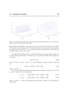
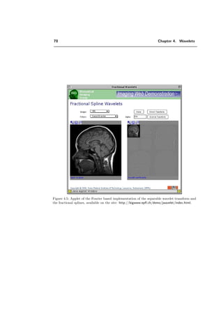
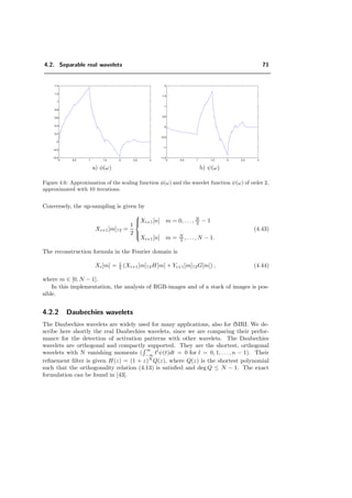
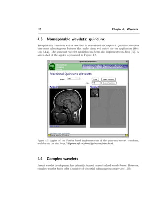
![2
↑ H(z)
Figure 4.2: Synthesis part of the 1D discrete wavelet transform (IDWT) for two iterations.
Let x[k] denote a one dimensional discrete signal. Then its down-sampled version
with 2 is
[x]↓2[k] = x[2k]. (4.27)
The Fourier-domain version of (4.27) is
[x]↓2[k] ←→
1
2
X z
1
2 + X −z
1
2 .
The up-sampling is defined by
[x]↑2[k] =
x[l] k = 2l, k even
0 k odd
and its effect in the transform domain is as follows:
[x]↑2[k] ←→ X z2
.
If we now chain the down-sampling and up-sampling operators, we obtain
[x]↓2↑2[k] =
x[k] k even
0 k odd
1
2
[X (z) + X (−z)] . (4.28)
The low-pass filter H reduces the resolution by a factor of 2; the wavelet coefficients
correspond to the output of the high-pass filter G. Applying the relation (4.28) to the
block diagram in Fig. 4.3, it is easy to derive the conditions for a perfect reconstruction:
H (z) H (z) + G (z) G (z) = 2 no distortion,
H (−z) H (z) + G (−z) G (z) = 0 alias cancellation.
(4.29)](https://image.slidesharecdn.com/0eba55bf-42a7-4963-8f0c-60b852f024ac-160911124222/85/feilner0201-83-320.jpg)
![66 Chapter 4. Wavelets
xi[k]
˜G (z)](https://image.slidesharecdn.com/0eba55bf-42a7-4963-8f0c-60b852f024ac-160911124222/85/feilner0201-84-320.jpg)
![2
↓
yi+1[k]
˜H (z)](https://image.slidesharecdn.com/0eba55bf-42a7-4963-8f0c-60b852f024ac-160911124222/85/feilner0201-85-320.jpg)
![2
↓
xi+1[k]
xi[k]](https://image.slidesharecdn.com/0eba55bf-42a7-4963-8f0c-60b852f024ac-160911124222/85/feilner0201-86-320.jpg)
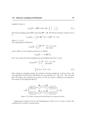
![2
↑ H (z)
Figure 4.3: Perfect reconstruction filterbank.
4.2 Separable real wavelets
By separable wavelets, we mean here separable filters and separable sampling. In the
two-dimensional case, the filters are obtained through the scaling function
φ(x, y) = φ(x)φ(y). (4.30)
In the two-dimensional case, we obtain this way three basic wavelets,
ψ1(x, y) = φ(x)ψ(y)
ψ2(x, y) = ψ(x)φ(y)
ψ3(x, y) = ψ(x)ψ(y).
Sampling in multiple dimensions is represented by a lattice, the set of all vectors generated
by Dk, k ∈ Zn
, where D is the matrix characterizing the sampling process. D is not
unique for a given sampling pattern [48]. A separable lattice is a lattice that can be
represented by a diagonal matrix. In two dimensions, the dyadic sampling matrix has
the expression
D =
2 0
0 2
.
The separable 2D wavelet transform has four outputs: one low-pass and three high-pass
branches.
The advantage of using a separable wavelet transform is twofold. First, it is simpler since
the 1D approach can be extended to higher dimensions through the use of tensor product
basis functions. The second reason is that separability is computationally more efficient,
since the transform can be implemented by treating the rows and columns separately.
The tensor product solution has the disadvantage that the filters obtained in this way
have a constrained design (nonseparable filters of size N1 × N2 would offer N1N2 free
design variables versus N1 + N2 in the separable case). The second drawback is that
only rectangular divisions of the spectrum are possible. It is usually the case that other
divisions may better capture the signal energy [148].](https://image.slidesharecdn.com/0eba55bf-42a7-4963-8f0c-60b852f024ac-160911124222/85/feilner0201-88-320.jpg)
![4.2. Separable real wavelets 67
4.2.1 Fractional splines
We describe here the discrete wavelet transform that arises from a multiresolution anal-
ysis generated by fractional splines. Fractional splines are a generalization of B-splines
to fractional orders. B-splines are constructed from the (n − 1)-fold convolution of a
rectangular pulse β0
+ [144]:
β0
+(x) =
1, 0 x 1
0, otherwise
(4.31)
βn
+(x) = β0
+ ∗ β0
+ ∗ · · · ∗ β0
+(x)
(n+1) times
. (4.32)
For n integers, these functions have a central axis of symmetry around n+1
2 , and can be
re-centered to yield the symmetric B-splines:
βn
∗ (x) = βn
+ x +
n + 1
2
. (4.33)
Likewise there are two flavors of fractional splines: the causal ones, denoted by βα
+, which
are a linear combination of the one-sided power functions
(x − n)α
+ =
(x − n)α
, x ≥ n
0, x n
; (4.34)
and the symmetric ones, denoted by βα
∗ , which are a linear combination of the radial
power functions |x − n|α
if α is any non-even real number, and of |x − n|α
log |x − n| if
α is even. For each version, the degree α of the splines is assumed to be strictly greater
than −1
2 , in order to ensure a valid MRA [135].
These functions have a simple expression in the frequency domain:
ˆβα
+(ω) =
1 − e−jω
jω
α+1
(4.35)
and ˆβα
∗ (ω) = |ˆβα
+(ω)|. They satisfy two-scale difference equations whose scaling filters
are given, respectively, by
Bα
+(z) =
√
2
1 + z−1
2
α+1
(4.36)
for the causal spline, and by
Bα
∗ (z) =
√
2
1 + z−1
2
α+1
(4.37)](https://image.slidesharecdn.com/0eba55bf-42a7-4963-8f0c-60b852f024ac-160911124222/85/feilner0201-89-320.jpg)
![68 Chapter 4. Wavelets
for the symmetric one.
The autocorrelation filter of a B-spline of degree α is given by
Aα
(ejω
) =
n
ˆβα
∗ (ω + 2nπ)
2
. (4.38)
Letting Bα
= Bα
+ or Bα
∗ , the discrete Fractional Spline Wavelet Transform (FSWT) is
implemented using the analysis and synthesis filters given in Table 4.1. Note that the
b
b
bbfilter
type
bspline ortho dual
H(z) Bα
(z) Bα
(z)
Aα(z)
Aα(z2)
Bα
(z−1
)
Aα
(z)
Aα (z2)
G(z) −z−1
Bα
(−z−1
)Aα
(−z) −z−1
Bα
(−z−1
)
Aα (−z)
Aα (z2)
−zBα
(−z)
Aα (z2)
H(z) Bα
(z−1
)
Aα
(z)
Aα (z2)
Bα
(z−1
)
Aα (z)
Aα (z2)
Bα
(z)
G(z)
−zBα
(−z)
Aα (z2)
−zBα
(−z)
Aα(−z)
Aα(z2)
−z−1
Bα
(−z−1
)Aα
(−z)
Table 4.1: Analysis and synthesis filters for the wavelet transform.
dual type is obtained by exchanging the analysis- and synthesis-part of the bspline case.
In Figure 4.4, the low-pass filter H(z) of the symmetric orthogonal fractional spline is
presented for different order parameters α. With increasing α, the filter is less local in
space but more frequency selective.
Implementation in Fourier
We have worked out a fast and exact implementation of the FSWT in 2D and 3D in the
Fourier domain based on [20]. The MATLAB files are freely available on our website1
.
We have also an FFT-based implementation of the FSWT in Java 2.0 [70]. The
principal advantage of Java over C++ is portability; indeed, there are now widely avail-
able virtual Java machines for most workstations including Mac, PC, and Sun. The
final form of the algorithm is a plugin implemented in Java for ImageJ [114], a Java
free-software available on the site of the National Institute of Health (NIH). The other
final form is an applet, which makes it possible to run the algorithm over the Inter-
net. A screen-shot of this applet is presented in Figure 4.5 and is available on the site
http://bigwww.epfl.ch/demo/jwavelet/index.html. The performance of the algorithm is as
1http://bigwww.epfl.ch/blu/fractsplinewavelets/](https://image.slidesharecdn.com/0eba55bf-42a7-4963-8f0c-60b852f024ac-160911124222/85/feilner0201-90-320.jpg)
![4.2. Separable real wavelets 69
0.5
1
1.5
2
2.5
3
3.5
4
10
5
0
-5
-10
-0.5
0
0.5
1
α
0.5
1
1.5
2
2.5
3
3.5
4
0.5
0
-0.5
0
0.5
1
1.5
α
a) b)
Figure 4.4: a) Impulse response of the orthogonal fractional spline dependent on α. b) Frequency
response of the orthogonal fractional spline.
follows (Pentium 500 MHz): an image of size of 512 × 512, 32-bits takes for one iteration
1.10 s and for nine iterations 1.30 s. The implementation has been conceived to minimize
the number and size of FFT’s. In the present version, the calculation of the FFT and
the IFFT takes up 50 % of the time.
The algorithm is implemented in a separable fashion and the intermediate results are
stored in floating point format. The first step is to perform the FFT of the signal (row
or column):
xi[k]
FFT
←→ Xi[n] (4.39)
where k ∈ [0, N − 1] and n ∈ [0, N − 1]. Down-sampling in Fourier domain is achieved
by
Xi[n]↓2 = 1
2 Xi[n] + Xi[n + N
2 ] , (4.40)
where n ∈ [0, N
2 − 1].
Thus, the two down-sampled filtered components in the Fourier domain (Xi+1[n] and
Yi+1[n], cf. Figure 4.3) are computed as
Xi+1[n] = 1
2 Xi[n]H[n] + Xi[n + N
2 ]H[n + N
2 ] (4.41)
Yi+1[n] = 1
2 Xi[n]G[n] + Xi[n + N
2 ]G[n + N
2 ] , (4.42)
where n ∈ [0, N
2 − 1]. The corresponding N
2 -point signals in Figure 4.3 are obtained by
inverse FFT.](https://image.slidesharecdn.com/0eba55bf-42a7-4963-8f0c-60b852f024ac-160911124222/85/feilner0201-91-320.jpg)
![4.2. Separable real wavelets 71
0 0.5 1 1.5 2 2.5 3
−0.4
−0.2
0
0.2
0.4
0.6
0.8
1
1.2
1.4
0 0.5 1 1.5 2 2.5 3
−1.5
−1
−0.5
0
0.5
1
1.5
2
a) φ(ω) b) ψ(ω)
Figure 4.6: Approximation of the scaling function φ(ω) and the wavelet function ψ(ω) of order 2,
approximated with 10 iterations.
Conversely, the up-sampling is given by
Xi+1[m]↑2 =
1
2
Xi+1[n] m = 0, . . . , N
2 − 1
Xi+1[n] m = N
2 , . . . , N − 1.
(4.43)
The reconstruction formula in the Fourier domain is
Xi[m] = 1
2 (Xi+1[m]↑2H[m] + Yi+1[m]↑2G[m]) , (4.44)
where m ∈ [0, N − 1].
In this implementation, the analysis of RGB-images and of a stack of images is pos-
sible.
4.2.2 Daubechies wavelets
The Daubechies wavelets are widely used for many applications, also for fMRI. We de-
scribe here shortly the real Daubechies wavelets, since we are comparing their perfor-
mance for the detection of activation patterns with other wavelets. The Daubechies
wavelets are orthogonal and compactly supported. They are the shortest, orthogonal
wavelets with N vanishing moments (
∞
−∞
tl
ψ(t)dt = 0 for l = 0, 1, . . ., n − 1). Their
refinement filter is given H(z) = (1 + z)N
Q(z), where Q(z) is the shortest polynomial
such that the orthogonality relation (4.13) is satisfied and deg Q ≤ N − 1. The exact
formulation can be found in [43].](https://image.slidesharecdn.com/0eba55bf-42a7-4963-8f0c-60b852f024ac-160911124222/85/feilner0201-93-320.jpg)
![72 Chapter 4. Wavelets
4.3 Nonseparable wavelets: quincunx
The quincunx transform will be described in more detail in Chapter 5. Quincunx wavelets
have some advantageous features that make them well suited for our application (Sec-
tion 7.2.2). The quincunx wavelet algorithm has been also implemented in Java [77]. A
screen-shot of the applet is presented in Figure 4.7.
Figure 4.7: Applet of the Fourier based implementation of the quincunx wavelet transform,
available on the site: http://bigwww.epfl.ch/demo/jquincunx/index.html.
4.4 Complex wavelets
Recent wavelet development has primarily focused on real-valued wavelet bases. However,
complex wavelet bases offer a number of potential advantageous properties [159]:](https://image.slidesharecdn.com/0eba55bf-42a7-4963-8f0c-60b852f024ac-160911124222/85/feilner0201-94-320.jpg)
![4.5. Applications 73
1 2 3 4 5 6
−0.2
0
0.2
0.4
0.6
0.8
k
h[k]
1 2 3 4 5 6
−1
−0.5
0
0.5
1
kg[k]
(a) (b)
Figure 4.8: Complex Daubechies filters. The solid line represents the real part, the dashed line
represents the imaginary part. a) h[k] for complex Daubechies of order 3. b) g[k] for complex
Daubechies of order 3.
− Daubechies has shown that all compactly supported, real orthogonal wavelet bases
and their associated conjugate quadrature filter (CQF) filterbanks are neither sym-
metric nor antisymmetric, except for the Haar transform [43, 42]. Lawton [88] and
Lina et al. [93] showed that symmetry could be regained by using complex scaling
functions. This led then to the definition of the Complex Daubechies wavelets,
which are symmetric, orthogonal and of minimum length. These wavelets have
been used in image coding applications in [16] and showed better compression per-
formance than asymmetric wavelets.
− Another advantage is the near shift-invariance of the complex wavelet transform
without significant increase of the complexity of the algorithm [118, 29]. The price
to pay is that the complex wavelet transform is redundant by a factor of two when
the input signal is real.
We also used the complex symmetric Daubechies wavelets for our fMRI application and
implemented the filters like described in [91, 92]. We implemented the order n = 3, 5, 7, 9.
The first order wavelet is the Haar wavelet. Note that the amplitude responses for the
complex real Daubechies filters are the same, see Figure 7.20. The filter coefficients h[k]
and g[k] for the order n = 3 are illustrated in Figure 4.8.
4.5 Applications
The wavelet transform is a powerful tool for many applications. Its space-frequency
localization property and the existence of fast algorithms make it attractive for the anal-](https://image.slidesharecdn.com/0eba55bf-42a7-4963-8f0c-60b852f024ac-160911124222/85/feilner0201-95-320.jpg)
![74 Chapter 4. Wavelets
ysis of non-stationary signals. The space-frequency localization property motivates new
algorithms for example for image denoising applications, where the wavelet transform is
able to preserve boundaries better than, for example, the Fourier transform [5, 72].
Another advantage of the wavelet transform as compared to the Fourier transform, is
that the analyzing wavelet can be specifically tailored to the application. The Windowed
Fourier Transform (WFT) circumvents the lack of time localization of the Fourier trans-
form, however, it remains the problem of the fixed size of each shifted window, whereas
for the wavelet transform we have different scales.
But also the scale specific non-redundant information of the wavelet coefficient makes the
wavelet transform attractive. For detection problems like fMRI or microcalcifications in
mammography, where the size of the feature to detect is not known a priori, the multires-
olution properties of the wavelet transform give access to signal information at different
resolution levels. This allows for the separation of signal components of various sizes
including high frequency noise. Another example than fMRI of successful application is
the detection of microcalcifications [158, 35].
The wavelet transform also de-correlates the signal, which results in a concentration of
power into a smaller number of coefficients. This makes the wavelet transform espe-
cially attractive for the compression of signals or images. Wavelets have already been
incorporated into the new JPEG2000 algorithm; they tend to be quite flexible and yield
subjectively better results than the standard DCT-based JPEG, at especially high com-
pression ratios.
Here, we will apply the wavelet transform to fMRI data.](https://image.slidesharecdn.com/0eba55bf-42a7-4963-8f0c-60b852f024ac-160911124222/85/feilner0201-96-320.jpg)
![Chapter 5
Orthogonal Quincunx Wavelets
with Fractional Orders
In this chapter, we present a new family of 2D and 3D orthogonal wavelets which uses
quincunx sampling. The orthogonal refinement filters have a simple analytical expression
in the Fourier domain as a function of the order λ, which may be non-integer. We can
also prove that they yield wavelet bases of L2(R2
) for any λ 0. The wavelets are
fractional in the sense that the approximation error at a given scale a decays like O(aλ
);
they also essentially behave like fractional derivative operators. To make our construction
practical, we propose an FFT-based implementation that turns out to be surprisingly
fast. In fact, our method is almost as efficient as the standard Mallat algorithm for
separable wavelets.
5.1 Introduction
The great majority of wavelet bases that are currently used for image processing are sep-
arable. There are two primary reasons for this. The first is convenience because wavelet
theory is most developed in 1D and that these results are directly transposable to higher
dimensions through the use of tensor product basis functions. The second is efficiency be-
cause a separable transform can be implemented by successive 1D processing of the rows
and columns of the image. The downside, however, is that separable transforms tend to
privilege the vertical and horizontal directions. They also produce a so-called “diagonal”
wavelet component, which does not have a straightforward directional interpretation.
Non separable wavelets, by contrast, offer more freedom and can be better tuned
to the characteristics of images [82, 103]. Their less attractive side is that they require
more computations. The quincunx wavelets are especially interesting because they can](https://image.slidesharecdn.com/0eba55bf-42a7-4963-8f0c-60b852f024ac-160911124222/85/feilner0201-97-320.jpg)
![76 Chapter 5. Orthogonal Quincunx Wavelets with Fractional Orders
be designed to be nearly isotropic [56]. In contrast with the separable case, there is a
single wavelet and the scale reduction is more progressive: a factor
√
2 instead of 2. The
preferred technique for designing quincunx wavelets with good isotropy properties is to
use the McClellan transform to map 1D biorthogonal designs to the multidimensional
case [99]. Since this approach requires the filters to be symmetric, it has only been
applied to the biorthogonal case because of the strong incentive to produce filters that
are compactly supported [31, 81, 125, 138].
In this chapter, we construct a new family of quincunx wavelets that are orthogonal
and have a fractional order of approximation. The idea of fractional orders was intro-
duced recently in the context of spline wavelets for extending the family to non-integer
degrees [145]. The main advantage of having a continuously-varying order parameter—
not just integer steps as in the traditional wavelet families—is flexibility. It allows for
a continuous adjustment of the key parameters of the transform; e.g., regularity and
localization of the basis functions. The price that we are paying for these new features—
orthogonality with symmetry as well as fractional orders—is that the filters can no longer
be compactly supported. We will make up for this handicap by proposing a fast FFT-
based implementation which is almost as efficient as Mallat’s algorithm for separable
wavelets [95].
5.2 Quincunx sampling and filterbanks
k1
k2
(a)
−π ω1
ω2
π
(b)
Figure 5.1: The quincunx lattice (a) and its corresponding bandwidth (b).
First, we recall some basic results on quincunx sampling and perfect reconstruction
filterbanks [148]. The quincunx sampling lattice is shown in Fig. 5.1. Let x[k] with
k = (k1, k2) ∈ Z2
denote the discrete signal on the initial grid. The 2D Fourier transform
of x[k] is denoted by X(ω) = k∈Z2 x[k]e−j ω,k
with ω = (ω1, ω2). Then, its quincunx](https://image.slidesharecdn.com/0eba55bf-42a7-4963-8f0c-60b852f024ac-160911124222/85/feilner0201-98-320.jpg)
![5.2. Quincunx sampling and filterbanks 77
sampled version is
[x]↓D[k] = x[Dk] where D =
1 1
1 −1
. (5.1)
Our down-sampling matrix D is such that D2
= 2I. The Fourier-domain version of (5.1)
is
[x]↓D[k] ←→
1
2
X D−T
ω + X D−T
ω + π ,
where π = (π, π).
The upsampling is defined by
[x]↑D[k] =
x[D−1
k] if k1 + k2 even
0 else where
and its effect in the transform domain is as follows:
[x]↑D[k] ←→ X DT
ω .
If we now chain the down-sampling and up-sampling operators, we get
[x]↓D↑D[k] =
x[k] if k1 + k2 even
0 else where
1
2
[X (ω) + X (ω + π)] . (5.2)
Since quincunx sampling reduces the number of image samples by a factor of two, the
corresponding reconstruction filterbank has two channels (cf. Fig. 5.2). The low-pass
filter H reduces the resolution by a factor of
√
2; the wavelet coefficients correspond to
the output of the high-pass filter G.
xi[k]
˜G (ω)](https://image.slidesharecdn.com/0eba55bf-42a7-4963-8f0c-60b852f024ac-160911124222/85/feilner0201-99-320.jpg)
![D
↓
yi+1[k]
˜H (ω)](https://image.slidesharecdn.com/0eba55bf-42a7-4963-8f0c-60b852f024ac-160911124222/85/feilner0201-100-320.jpg)
![D
↓
xi+1[k]
xi[k]](https://image.slidesharecdn.com/0eba55bf-42a7-4963-8f0c-60b852f024ac-160911124222/85/feilner0201-101-320.jpg)
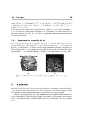
![78 Chapter 5. Orthogonal Quincunx Wavelets with Fractional Orders
H (ω) H (ω) + G (ω) G (ω) = 2
H (ω + π) H (ω) + G (ω + π) G (ω) = 0,
(5.3)
where H and G (resp., H and G) are the transfer functions of the synthesis (resp.,
analysis) filters. In the orthogonal case, the analysis and synthesis filters are identical up
to a central symmetry; the wavelet filter G is simply a modulated version of the low-pass
filter H.
5.3 Fractional quincunx filters
To generate quincunx filters, we will use the standard approach which is to apply the
diamond McClellan transform to map a one dimensional design onto the quincunx struc-
ture.
5.3.1 A new 1D wavelet family
As starting point for our construction, we introduce a new one-dimensional family of
orthogonal filters:
Hλ(z) =
√
2(z + 2 + z−1
)
λ
2
(z + 2 + z−1)λ + (−z + 2 − z−1)λ
=
√
2(2 + 2 cosω)
λ
2
(2 + 2 cosω)λ + (2 − 2 cos ω)λ
, (5.4)
which is indexed by the continuously-varying order parameter λ.
These filters are symmetric and are designed to have zeros of order λ at z = −1; the
numerator is a fractional power of (z+2+z−1
) (the simplest symmetric refinement filter)
and the denominator is the appropriate orthonormalization factor. By varying λ, we can
adjust the frequency response as shown in Fig. 5.3. As λ increases, Hλ(z) converges to
the ideal half-band low-pass filter. Also note that these filters are maximally flat at the
origin; they essentially behave like Hλ (ω) /
√
2 = 1 + O(ωλ
) as ω → 0. Their frequency
response is similar to the Daubechies’ filters with two important differences: (1) the
filters are symmetric, and (2) the order is not restricted to integer values.
We can prove mathematically that these filters will generate valid 1D fractional
wavelet bases of L2 similar to the fractional splines presented in [145]. The order property
(here fractional) is essential because it determines the rate of decay of the approximation
error as a function of the scale. It also conditions the behavior of the corresponding
wavelet which will act like a fractional derivative of order λ; in other words, it will kill
all polynomials of degree n ≤ λ − 1 .](https://image.slidesharecdn.com/0eba55bf-42a7-4963-8f0c-60b852f024ac-160911124222/85/feilner0201-104-320.jpg)
![5.3. Fractional quincunx filters 79
0 0.1 0.2 0.3 0.4 0.5
0
0.5
1
1.5
Normalized Frequency
Amplitude
Figure 5.3: Frequency responses of the orthogonal refinement filters for λ = 1, . . . , 100.
5.3.2 Corresponding 2D wavelet family
Applying the diamond McClellan transform to the filter above is straightforward; it
amounts to replacing cos ω by 1
2 (cos ω1 + cosω2) in (5.4). Thus, our quincunx refinement
filter is given by
Hλ(ω1, ω2) =
√
2(2 + cos ω1 + cos ω2)
λ
2
(2 + cos ω1 + cos ω2)λ + (2 − cos ω1 − cos ω2)λ
. (5.5)
This filter is guaranteed to be orthogonal because the McClellan transform has the
property of preserving biorthogonality. Also, by construction, the λth order zero at ω = π
gets mapped into a corresponding zero at (ω1, ω2) = (π, π); this is precisely the condition
that is required to get a two dimensional wavelet transform of order λ.
The orthogonal wavelet filter is obtained by modulation
Gλ(ω1, ω2) = ejω1
Hλ(−ω1 − π, −ω2 − π). (5.6)
The corresponding orthogonal scaling function ϕλ (x) is defined implicitly as the
solution of the quincunx two-scale relation:
ϕλ (x) =
√
2
k∈Z2
hλ[k]ϕλ Dx − k .
Since the refinement filter is orthogonal with respect to the quincunx lattice, it follows
that ϕλ (x) ∈ L2(R2
) and that it is orthogonal to its integer translates. Moreover, for
λ 0, it will satisfy the partition of unity condition, which comes as a direct consequence](https://image.slidesharecdn.com/0eba55bf-42a7-4963-8f0c-60b852f024ac-160911124222/85/feilner0201-105-320.jpg)
![80 Chapter 5. Orthogonal Quincunx Wavelets with Fractional Orders
of the vanishing of the filter at (ω1, ω2) = (π, π). Thus, we have the guarantee that
our scheme will yield orthogonal wavelet bases of L2(R2
). The underlying orthogonal
quincunx wavelet is simply
ψλ (x) =
√
2
k∈Z2
gλ[k]ϕλ Dx − k .
5.4 Implementation in Fourier domain
xi[k]
˜G (ω)](https://image.slidesharecdn.com/0eba55bf-42a7-4963-8f0c-60b852f024ac-160911124222/85/feilner0201-106-320.jpg)
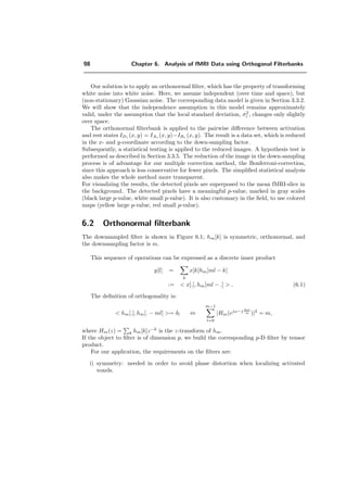
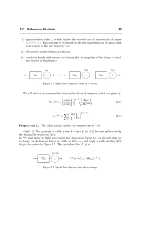
![2I
↓
h+ r zi+1[k]
˜H (ω)](https://image.slidesharecdn.com/0eba55bf-42a7-4963-8f0c-60b852f024ac-160911124222/85/feilner0201-110-320.jpg)
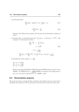
![D
↑
xi+1[k]
yi+1[k]
↑
↑
˜Gp (ω)](https://image.slidesharecdn.com/0eba55bf-42a7-4963-8f0c-60b852f024ac-160911124222/85/feilner0201-112-320.jpg)
![2I
↓ • yi+2[k]
˜Hp (ω)](https://image.slidesharecdn.com/0eba55bf-42a7-4963-8f0c-60b852f024ac-160911124222/85/feilner0201-113-320.jpg)
![2I
↓ • xi+2[k]
Figure 5.4: Analysis part of the 2D QWT for two iterations.
2
1y
y3
y4
x4
y
Figure 5.5: Formation of quincunx coefficients for 4 iterations.
The major objection that can be made to our construction is that the filters are not
FIR and that it may be difficult and costly to implement the transform in practice. We
will see here that we can turn the situation around and obtain a very simple and efficient
algorithm that is based on the FFT, following the idea of [117]. Working in the frequency
domain is also very convenient because of the way in which we have specified our filters](https://image.slidesharecdn.com/0eba55bf-42a7-4963-8f0c-60b852f024ac-160911124222/85/feilner0201-114-320.jpg)
![5.4. Implementation in Fourier domain 81
y1
y2 y3
y4 x4
Figure 5.6: Other possible formation of quincunx coefficients for 4 iterations.
(cf. Eqs. (5.5) and (5.6)). A first such implementation has been done by [104]. Our
algorithm is an other variation, which minimizes the number and size of FFT’s and seems
to be faster.
Here, we will only describe the decomposition part of our algorithm which corresponds
to the block diagram presented in Fig. 5.4 where we have pooled together two levels of
decomposition. The initialization step is to evaluate the FFT of the initial input image
x[k] and to precompute the corresponding sampled frequency responses of the analysis
filters H [n] and G [n] using (5.5) and (5.6).
Assuming that the current image size is N × N, the input variable, following a 2D
FFT, is
Xi [n] =
k
xi[k]e−j 2π k,n
N for n1, n2 = 0 . . . N − 1.
Globally, at the end of the process, the output variables are the quincunx wavelet
coefficients y1[k], y2[k], ..., yJ [k] and xJ [k] (see Fig. 5.5). Their Fourier transforms for
the odd iteration are derived from the auxiliary N × N signals:
Xi+1 [n] =
k
xi+1[k]e−j 2π k,n
N ,
Yi+1 [n] =
k
yi+1[k]e−j 2π k,n
N n1, n2 ∈ [0, N − 1]2
. (5.7)
Down- and upsampling with D in the first iteration step (see Figure 5.4) introduces
zeros in the space domain and preserves size (Yi+1[n]); however, it implies some symme-
try/redundancy in frequency domain. Only half of the coefficients need to be computed
which saves operations. This reduced signal Yi+1[k] and its corresponding low-pass signal](https://image.slidesharecdn.com/0eba55bf-42a7-4963-8f0c-60b852f024ac-160911124222/85/feilner0201-115-320.jpg)
![82 Chapter 5. Orthogonal Quincunx Wavelets with Fractional Orders
is obtained by
Yi+1 [m1, n2] = 1
2 G [m1, n2] Xi [m1, n2] (5.8)
+G m1 + N
2 , n2 + N
2 Xi m1 + N
2 , n2 + N
2
Xi+1 [m1, n2] = 1
2 H [m1, n2] Xi [m1, n2]
+H m1 + N
2 , n2 + N
2 Xi m1 + N
2 , n2 + N
2 ,
where m1 ∈ [0, N
2 − 1], n2 ∈ [0, N − 1].
To generate the signal yi+1[k] of (5.7) in the way that is depicted in Figure 5.5 with
every second row shifted by one pixel, we separate the image in even (yi+1,even) and odd
(yi+1,odd) rows already in the Fourier domain, using the auxiliary variable Z[m]:
Z[m] = Yi+1[m] + Yi+1 m + 0, N
2
+j Yi+1[m] − Yi+1 m + 0, N
2 ej
2π(m1+m2)
N
zi+1[k] = yi+1,even[k] + jyi+1,odd[k]. (5.9)
The sum in the real part (Yi+1[m] + Yi+1[m + 0, N
2 ]) represents downsampling by two,
keeping all the even rows, whereas the sum in the imaginary part represents the odd
rows.
In the space domain, we alternate the rows yi+1 [k1, 2k2 + 1] = Re z[k] and
yi+1 [k1, 2k2] = Im z[k] . Since z[k] is four times smaller than yi+1[k], we save compu-
tations with the reduced-size IFFT.
Instead of rotating the frequency variables after each iteration, we calculate a rotated
version of the filters H[z] → Hp[z] and G[z] → Gp[z], which we apply at all even itera-
tions. In this way, we also save two rotations per iteration in the frequency domain.
The Fourier transforms of the output for the even iterations are:
Yi+2 [m] = k yi+2[k]e
−j 2π k,m
N
2 for m1, m2 = 0 . . . N
2 − 1.
Its source is:
Xi+2 [m] = 1
2 Hp [m] Xi+1 [m] + Hp m + 0, N
2 Xi+1 m + 0, N
2 (5.10)
Yi+2 [m] = 1
2 Gp [m] Xi+1 [m] + Gp m + 0, N
2 Xi+1 m + 0, N
2 ,](https://image.slidesharecdn.com/0eba55bf-42a7-4963-8f0c-60b852f024ac-160911124222/85/feilner0201-116-320.jpg)
![5.5. Experiments 83
where Hp [m] = H [Dm mod (N, N)] and Gp [m] = G [Dm mod (N, N)]. The process
is then iterated until one reaches the final resolution. When the last iteration is even,
we lower the computation costs with the FFT by utilizing its imaginary part: z[k] =
m (Xi+2[m] + jYi+2[m]) e
j 2π m,k
N
2 , where xi+2[k] = Re z[k] and yi+2[k] = Im z[k] .
Obviously, as one gets coarser, the Fourier transforms of the filters need not be recalcu-
lated; they are simply obtained by down-sampling the previous arrays.
The synthesis algorithm operates according to the same principles and corresponds
to the flow graph transpose of the decomposition algorithm using up-sampling instead.
For instance, the synthesis counterpart of (5.10) is:
Xi+2 m1, m2 + N
2 = Xi+2 [m1, m2]
Yi+2 m1, m2 + N
2 = Yi+2 [m1, m2]
Xi+1 [m1, n2] = Xi+2[m1, n2]Hp[m1, n2] + Yi+2[m1, n2]Gp[m1, n2].
5.5 Experiments
5.5.1 Benchmark and testing
We have implemented the algorithm in Matlab and report computation times below
0.85 sec for four iterations and for a 256×256 image on an aging Sun Ultra 30 workstation;
the decomposition is essentially perfect with an (RMS) reconstruction error below 10−12
.
The method is generic and works for any set of filters that can be specified in the frequency
domain.
Two examples of fractional quincunx wavelet decompositions with λ =
√
2 and λ = π
are shown in Fig. 5.7. Note how the residual image details are more visible for the lower
value of λ. The larger λ reduces the energy of the wavelet coefficient, but this also comes
at the expense of some ringing. Thus, it is convenient to have an adjustable parameter
to search for the best tradeoff.
An advantage of the present approach is that the filters for small λ are nearly isotropic;
this is the reason why the wavelet details in Fig. 5.7 do not present any preferential
orientation. The degree of isotropy of the various filters can be visualized in Figure 5.8.
The shape of the contour-plots of the low-pass filter H(ω) confirms that the degree of
isotropy is the best for small values of λ. At the other extreme, when λ → ∞, H(ω)
tends to the diamond-shaped ideal filter.
Another nice feature of the algorithm is that the computational cost remains the same
irrespective of the value of λ.](https://image.slidesharecdn.com/0eba55bf-42a7-4963-8f0c-60b852f024ac-160911124222/85/feilner0201-117-320.jpg)
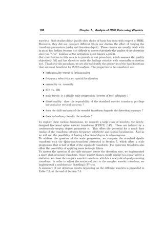
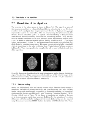
![86 Chapter 5. Orthogonal Quincunx Wavelets with Fractional Orders
5.5.2 Dependence of the order parameter
The usefulness of a tunable order parameter is demonstrated in the following experiment:
we apply the quincunx transform to an image (“cameraman”) and reconstruct the image
with only 15 % of the largest coefficients and measure then the SNR depending on
the order parameter. The graph 5.9 shows the SNR dependence on λ; the optimum is
achieved with λ = 2.1.
0 5 10 15
14
16
18
20
22
24
26
28
order parameter λ
SNR
Figure 5.9: Relation between the order parameter λ and the SNR of the reconstructed image
with only 10000 of the largest coefficients. The reconstruction with λ = 2.1 reaches the highest
SNR.
5.5.3 Approximation properties
The main differences between the quincunx (quin) and the conventional algorithm (sep)
is the finer scale progression and the nonseparability. To test the impact that this may
have on compression capability, we compared the approximation of quin and sep. Since
the wavelet transform is orthogonal, the approximation error (distortion) is equal to
D2
= x − ˆx 2
= y − ˆy 2
, where y are the wavelet coefficients, x is the input, ˆx and ˆy
is the estimated image. Also D2
in the space domain is equivalent to the sum of squares
of discarded wavelet coefficients [143].
Linear approximation
In classical rate-distortion theory, the coefficients are grouped into channels and coded
independently. In the orthogonal case, D2
is equivalent to the difference between the](https://image.slidesharecdn.com/0eba55bf-42a7-4963-8f0c-60b852f024ac-160911124222/85/feilner0201-120-320.jpg)
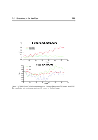
![88 Chapter 5. Orthogonal Quincunx Wavelets with Fractional Orders
signal’s energy and the energy of the reconstructed signal: x − ˆx 2
= x 2
− ˆx 2
=
x 2
− ˆxJ
2
+
J
j=1 ˆyj
2
. The distortion across J channels with variance σi is
D = J · C · 2−2 ¯R
· ρ2
,
where C is a constant, ¯R is the mean rate and ρ is the geometric mean of the subband
variances:
ρ =
J
i=1
σ2
i
1
J
.
When ρ is smaller, the distortion is smaller as well. What this means qualitatively is that
the wavelet transform which has the larger spread in the variances will achieve the better
coding gain [148]. The linear approximation subband coding gain for sample-by-sample
quantization (PCM) is described by:
GP CM =
DP CM
DSBC
=
1
J
J
i=1 σ2
i
J
i=1 σ2
i
1
J
.
In Figure 5.12 a) we compare the energy packing properties of quin and sep for linear
approximation. “Energy packing” refers to the property that the more the first coeffi-
cients contain energy, the better the DWT yields compression. We decomposed an image
I(x, y) for the maximal possible iteration J. The image I(x, y) is depicted in Figure 5.11;
its decompositions for quin and sep are shown on the right hand side. We start to sum
up the energy of the subbands with the lowest resolution. Each step of the stairs repre-
sents a subband. The first subbands of quin report higher energy than sep, as shown
in the Graph in Figure 5.12. Its coding gain for quin is GP CM = 77.9 and for sep
GP CM = 75.6. For the majority of images we considered, quin yielded better energy
packing than sep. However, we did also encounter one notable counter example, “Lena”,
(cf. Fig. 5.13), which seems to be better suited for a separable treatment.
Since the branches are orthogonal, the transformation that provides the maximum en-
ergy compaction in the low-pass channel is also the one that results in the minimum
approximation error [143]. Since most images have a power spectrum that is roughly
rotationally-invariant and decreases with higher frequencies, separable systems are usu-
ally not best suited for isolating a low-pass channel containing most energy and having
high-pass channels with low energy. In contrast, a quincunx low-pass filter will retain
more of the original signal’s energy [148].
Nonlinear approximation
A more recent trend in wavelet theory is the study of nonlinear approximation. In this
case we don’t take the “n-first” coefficients, but the “n-largest” coefficients to approxi-
mate a signal with n N coefficients. This yields better energy packing, since in the](https://image.slidesharecdn.com/0eba55bf-42a7-4963-8f0c-60b852f024ac-160911124222/85/feilner0201-122-320.jpg)
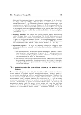
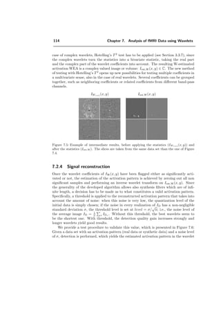
![5.6. Extension to 3D 91
k1
k2
k3
Figure 5.14: 3D-FCO (face-centered orthorhombic) lattice, corresponding to the sampling matrix
(5.11).
wavelet domain the “n-first” coefficients are not necessarily the largest one, especially
along the position-indices [47]. The distortion is described by [46]:
D2
= y − yN(T )
2
=
|y|T
|y[n]|2
.
Moreover, it can be shown that
D ∝ C · (N (T))− γ
2 ,
when the smoothness of y is measured by its inclusion in some critical Besov space
Bγ
q (Lq
(I)) with 1
q = γ
2 + 1
2 , roughly when y is a function with γ derivatives in Lq
(I).
For the nonlinear approximation, quin also yields a better approximation than sep for a
small n in many cases. Figure 5.12 b) represents the energy depending on the n largest
coefficients (in log). Further examples of (non-) linear examples are shown in Figure 5.13.
5.6 Extension to 3D
The extension of quincunx sampling to 3D is straight forward. The quincunx sampling
lattice for 3D is shown in Fig. 5.14. Let x[k] denote the discrete signal on the initial grid.
Then, its quincunx sampled version is
[x]↓D[k] = x[Dk] where D =
1 0 1
−1 −1 1
0 −1 0
. (5.11)](https://image.slidesharecdn.com/0eba55bf-42a7-4963-8f0c-60b852f024ac-160911124222/85/feilner0201-125-320.jpg)
![92 Chapter 5. Orthogonal Quincunx Wavelets with Fractional Orders
Our down-sampling matrix D is such that D3
= 2I and | det D| = 2. The Fourier-
domain version of this formula is similar to the case in 2D:
[x]↓D[k] ←→
1
2
X D−T
ω + X D−T
ω + π ,
where π = (π, π, π).
The implementation for 3D is as follows:
The output variables are the discrete Fourier transforms of the wavelet coefficients
Yi+1 [n] =
k
yi+1[k]e−j
2π k,n
N for n1, n2, n3 = 0 . . . N − 1
Yi+2 [n] =
k
yi+2[k]e−j 2π k,n
N for n1, n2, n3 = 0 . . . N − 1
Yi+3 [m] =
k
yi+3[k]e
−j
2π k,m
N
2 for m1, m2, m3 = 0 . . .
N
2
− 1
The coefficients themselves are recovered by inverse FFT. The Fourier transforms after
the first level of filtering are given by
Xi+1 [n] =
1
2
H [n] Xi [n] + H n +
N
2
,
N
2
,
N
2
Xi n +
N
2
,
N
2
,
N
2
Yi+1 [n] =
1
2
G [n] Xi [n] + G n +
N
2
,
N
2
,
N
2
Xi n +
N
2
,
N
2
,
N
2
.
After the second level of filtering, we have:
Xi+2 [n] =
1
2
Hp [n] Xi+1 [n] + Hp n + 0,
N
2
, 0 Xi+1 n + 0,
N
2
, 0
Yi+2 [n] =
1
2
Gp [n] Xi+1 [n] + Gp n + 0,
N
2
, 0 Xi+1 n + 0,
N
2
, 0 .
Note that these are computed at the resolution of the input. The size reduction only
takes place during the third step:
Xi+3 [m] =
1
2
Hpp [m] Xi+2 [m] + Hpp m +
N
2
, 0, 0 Xi+2 m +
N
2
, 0, 0
Yi+3 [m] =
1
2
Gpp [m] Xi+2 [m] + Gpp m +
N
2
, 0, 0 Xi+2 m +
N
2
, 0, 0 ,](https://image.slidesharecdn.com/0eba55bf-42a7-4963-8f0c-60b852f024ac-160911124222/85/feilner0201-126-320.jpg)
![5.7. Conclusion 93
where Hp [m] = H [Dm mod (N, N, N)] and Hpp [m] = H D2
m mod (N, N, N) .
Analogously, we have that: Gp [m] = G [Dm mod (N, N, N)] and Gpp [m] =
G D2
m mod (N, N, N) .
It is still possible to optimize this implementation, especially for the calculation of FFT’s.
Also the redundancy for the second iteration may be removed. For reason of calculation
time, the computation of Hp, Hpp, Gp and Gpp as well the corresponding analysis filters
are implemented in C.
5.6.1 Approximation properties in 3D
We compared the compression capability for quin and sep for 3D-images, similar to
what is described for 2D in Section 5.5.3. An example is the volume V (x, y, z) depicted in
Figure 5.15 (human head). In Figure 5.16 are the graphs which represents the percentage
of the energy of V (x, y, z) (y-axis) corresponding to the number of coefficients, which
approximate V (x, y, z) (x-axis). Another example of this issue is shown in Figure 5.17.
(a) (b)
Figure 5.15: Volume V (x, y, z): a) surface of V (x, y, z) b) one slice of V (x, y, z).
5.7 Conclusion
We have introduced a new family of orthogonal wavelet transforms for quincunx lattices.
A key feature is the continuously-varying order parameter λ which can be used to adjust
the bandpass characteristics as well as the localization of the basis functions.
We have also demonstrated that these wavelet transforms could be computed quite ef-
ficiently using FFTs. This should help dispel the commonly held belief that non separable
wavelet decompositions are computationally much more demanding than the separable
ones.](https://image.slidesharecdn.com/0eba55bf-42a7-4963-8f0c-60b852f024ac-160911124222/85/feilner0201-127-320.jpg)
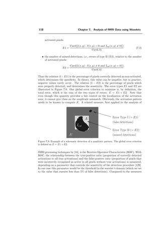
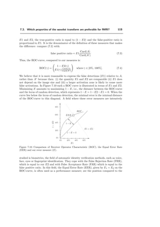
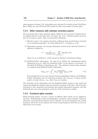
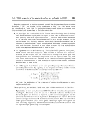
![98 Chapter 6. Analysis of fMRI Data using Orthogonal Filterbanks
Our solution is to apply an orthonormal filter, which has the property of transforming
white noise into white noise. Here, we assume independent (over time and space), but
(non-stationary) Gaussian noise. The corresponding data model is given in Section 3.3.2.
We will show that the independence assumption in this model remains approximately
valid, under the assumption that the local standard deviation, σ2
i , changes only slightly
over space.
The orthonormal filterbank is applied to the pairwise difference between activation
and rest states IDτ (x, y) = IAτ (x, y)−IBτ (x, y). The result is a data set, which is reduced
in the x- and y-coordinate according to the down-sampling factor.
Subsequently, a statistical testing is applied to the reduced images. A hypothesis test is
performed as described in Section 3.3.5. The reduction of the image in the down-sampling
process is of advantage for our multiple correction method, the Bonferroni-correction,
since this approach is less conservative for fewer pixels. The simplified statistical analysis
also makes the whole method more transparent.
For visualizing the results, the detected pixels are superposed to the mean fMRI-slice in
the background. The detected pixels have a meaningful p-value, marked in gray scales
(black large p-value, white small p-value). It is also customary in the field, to use colored
maps (yellow large p-value, red small p-value).
6.2 Orthonormal filterbank
The downsampled filter is shown in Figure 6.1; hm[k] is symmetric, orthonormal, and
the downsampling factor is m.
This sequence of operations can be expressed as a discrete inner product
y[l] =
k
x[k]hm[ml − k]
:= x[.], hm[ml − .] . (6.1)
The definition of orthogonality is:
hm[.], hm[. − ml] = δl ⇔
m−1
l=0
|Hm(ejω−j 2πl
m )|2
= m,
where Hm(z) = k hm[k]z−k
is the z-transform of hm.
If the object to filter is of dimension p, we build the corresponding p-D filter by tensor
product.
For our application, the requirements on the filters are:
i) symmetry: needed in order to avoid phase distortion when localizing activated
voxels.](https://image.slidesharecdn.com/0eba55bf-42a7-4963-8f0c-60b852f024ac-160911124222/85/feilner0201-132-320.jpg)
![6.2. Orthonormal filterbank 99
ii) approximation order λ (which implies the reproduction of polynomials of degree
≤ n = λ−1). This property is beneficial for a better approximation of signals with
most energy in the low frequency part.
iii) all possible integer decimation factors.
iv) consistent family with respect to chaining (for the simplicity of the design → mod-
ular library of transforms):
x hm
m
↓ y ⇐⇒ x hm1
m1
↓ hm2
m2
↓ y
Figure 6.1: Signal flow diagram, where m = m1m2.
We will use the orthonormal fractional spline filters of degree α, which are given by
Hm(ejω
) =
sin(mω
2 )
m sin(ω
2 )
α+1
A(ejω)
A(ejmω)
(6.2)
A(ejω
) =
k∈Z
sin(ω
2 )
(ω
2 + kπ)
2(α+1)
(6.3)
Proposition 6.1 The spline family satisfies the requirements i)—iv).
Proof. ii) This property is valid, where λ = α + 1 in (6.2) because splines satisfy
the Strang-Fix conditions [134].
iv) We start from the right-hand signal flow diagram in Figure 6.1. In the first step, we
exchange the decimation factor m1 with the filter hm2 and apply a noble identity [148]
to get the system in Figure 6.2. The equivalent filter G(z) is:
x G(z)
m1m2
↓ y G(z) = Hm1 (z)Hm2 (zm1
)
Figure 6.2: Signal flow diagram after the exchange.](https://image.slidesharecdn.com/0eba55bf-42a7-4963-8f0c-60b852f024ac-160911124222/85/feilner0201-133-320.jpg)
![100 Chapter 6. Analysis of fMRI Data using Orthogonal Filterbanks
G(ejω
) =
sin(m1
ω
2 )
m1 sin(ω
2 )
α+1
A(ejω)
A(ejm1ω)
sin(m1m2
ω
2 )
m2 sin(m1
ω
2 )
α+1
A(ejm1ω)
A(ejm1m2ω)
=
sin(m1
ω
2 )
m1 sin(ω
2 )
sin(m1m2
ω
2 )
m2 sin(m1
ω
2 )
α+1
A(ejω)
A(ejm1ω)
A(ejm1ω)
A(ejm1m2ω)
. (6.4)
After cancellation of common factors, we get:
G(ejω
) =
sin(m1m2
ω
2 )
m1m2 sin(ω
2 )
α+1
A(ejω)
A(ejm1m2ω)
= Hm1·m2 (ejω
). (6.5)
The proof that an orthogonal filter preserves the white noise is given in Section 6.4.
We also show that the “model 2” given in Section 3.3.2 remains approximately valid: If
the variance varies only slightly over the size of the filter, then the noise is still reasonably
independent.
6.3 Comparison of Gaussian versus orthogonal filter
Given an orthogonal filter with a decimation factor of m, we want to determine an
“equivalent” Gaussian filter which has exactly the same noise reduction power. The
notations are as follows:
i) x[.] : input signal, white noise with σ2
= 1 and µ = 0 (N(0, 1)).
ii) g[.] : filter coefficients.
iii) y[.] : output signal after filtering.
In general: y[n] = k g[n − k]x[k] with n g[n] = 1. The variance is:
E y2
[n] =
n k
g[k]x[n − k]
l
g[l]x[n − l]
=
k l
g[k]g[l]
n
x[n − k]x[n − l]
=
k l
g[k]g[l]δ[k − l]
=
k
g2
[k] (6.6)](https://image.slidesharecdn.com/0eba55bf-42a7-4963-8f0c-60b852f024ac-160911124222/85/feilner0201-134-320.jpg)
![6.4. Decorrelation property 101
• orthonormal filter:
k
g[nM − k]g[n M − k] =
1
M
δ[n − n ] (6.7)
⇒
k
g2
[k] =
1
M
(6.8)
Equation (6.8) follows from equation (6.7) because of the Strang-Fix condition of
order 1.
• Gaussian filter is normalized such that: n g[n] = 1 with g[n] = Ce
−n2
2σ2
. The
constant C is determined as follows:
n
e
−n2
2σ2
e
−x2
2σ2
dx
∼= σ
√
2π (6.9)
⇒ C
1
σ
√
2π
n
g2
[n] = C2
n
e
−n2
σ2
C2
e
−x2
σ2
dx = C2
σ
√
π =
1
2σ
√
π
• identification of the energies: σ = M
2
√
π
M = 2 : σ = 0.564
M = 4 : σ = 1.128
M = 8 : σ = 2.257
SPM recommends a Full Width of Half Maximum (FWHM) between 2 and 3. Since
FWHM = 2σ
√
2 log 2 and M =
√
π
√
2log(2)
FWHM, the range for the scaling factor is
3.0 ≤ M ≤ 4.5 and we obtain for M = 4 : FWHM = 2.66.
6.4 Decorrelation property
We prove here that an orthogonal filter transforms decorrelated noise into noise that is
essentially decorrelated as well. In particular, this means that it preserves white noise.](https://image.slidesharecdn.com/0eba55bf-42a7-4963-8f0c-60b852f024ac-160911124222/85/feilner0201-135-320.jpg)
![102 Chapter 6. Analysis of fMRI Data using Orthogonal Filterbanks
Theorem 6.4.1 Assume that the signal x[n] can be expressed as the sum of a deter-
ministic part, µ[n], and a non-stationary uncorrelated part b[n]. Let y[n] be the filtered
version of x[n], i.e., y[n] = h[n] ∗ x[n], where h[n] is orthonormal. If the fluctuations of
the standard deviation of b[n] are sufficiently small, then y[n] = h[n] ∗ µ[n] + z[n], where
E(z[n]z[n ]) ∼= σ2
δ[n − n ].
Proof.
input signal: x[n] = µ[n] + σ[n]e[n], where E [e[n]] = 0 and E [e[n]e[k]] = δ[n − k]
output signal: y[n] = k h[nM − k]x[k]
y[n] =
k
h[nM − k]µ[k]
ˆy[n]
+
k
h[nM − k]σ[k]e[k]
z[n] = y[n] − ˆy[n]
E[z[n]] = 0
E [z[n]z[n ]] = E
k
h[nM − k]σ[k]e[k]
k
h[n M − k ]σ[k ]e[k ]
=
k k
h[nM − k]h[n M − k ]σ[k]σ[k ] E [e[k]e[k ]]
δ[k−k ]
=
k
h[nM − k]h[n M − k]σ2
[k]
First case: uniform variance: σ[k] = σ:
E [z[n]z[n ]] = σ2
k
h[nM − k]h[n M − k]
1
M δ[n−n ], if h[n] is orthonormal
Second case: close to uniform variance: σ[k] = σ(1 + ε[k]), ε[k] 1
E [z[n]z[n ]] =
k
h[nM − k]h[n M − k]σ2
(1 + ε[k])2
= σ2
δ[n − n ] + σ2
k
h[nM − k]h[n M − k](2ε[k] + ε[k]2
)
r](https://image.slidesharecdn.com/0eba55bf-42a7-4963-8f0c-60b852f024ac-160911124222/85/feilner0201-136-320.jpg)
![6.5. Results 103
We bound the second term as follows:
r ≤
k
|h[nM − k]h[n M − k]|(sup 2|ε[k]| + sup ε[k]2
)
≤
k
h[nM − k]2
k
h[n M − k]2
= 1
M
(sup 2|ε[k]| + sup ε[k]2
) (Cauchy-Schwartz)
≤
1
M
sup 2|ε[k]| + sup ε[k]2
.
So that
E [z[n]z[n ]] = σ2
(δ[n − n ] + ρ[n, n ]),
where
|ρ[n, n ]| ≤
2
M
sup |ε[k]| + sup ε[k]2
1.
Thus, in both cases, z[n] remains essentially uncorrelated.
This theorem implies that the noise remains uncorrelated in every homogeneous zones
(σ = constant). However, the correlation property is not valid anymore on the border
of zones, like the border of the brain against the background, over a band that has the
width of the “efficient” length of the filter G.
6.5 Results
To illustrate the technique, we present some examples of real data analysis (cf. Figures 6.3
to 6.4). The data set is obtained from HUG and has the specification described in
Table 7.4. The task was watching a moving checker board of colors. After orthogonal
filtering and applying the Bonferroni-correction, we detect activity in the occipital lobe
(cf. Section 2.9). We also applied SPM [156] with a σ corresponding to the smoothing
factor of the orthogonal filter (Figure 6.3). The difference between our detection and
SPM is not negligible. The activation of the right hemisphere of the brain seems to be
comparable. However, in the left hemisphere, we detect an additional activation on the
border (cf. Figure 6.4). Applying a Gaussian filter of the same width as in SPM and
performing a t-test with Bonferroni-correction, we could confirm this detection. It is
unclear why SPM did not detect this pattern.
6.6 Conclusion
We have proposed a first approach that simplifies the statistical analysis of the data, as
compared to SPM. The idea is to continue “orthogonal” smoothing with down-sampling](https://image.slidesharecdn.com/0eba55bf-42a7-4963-8f0c-60b852f024ac-160911124222/85/feilner0201-137-320.jpg)
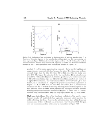
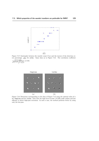
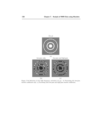
![Chapter 7
Analysis of fMRI Data using
Wavelets
7.1 Introduction
The use of the wavelet transform for the analysis of functional Magnetic Resonance
Imaging (fMRI) of the brain was pioneered by Ruttimann et al. [120]. The advantages
of this method over the more conventional spatial approaches are twofold. First, the
wavelet transform has a compression effect because it tends to pack the signal of interest
into a relatively few number of large coefficients. On the other hand, the noise gets
diluted evenly in the wavelet domain (provided the wavelet is close to orthogonal). This
results in an increase of the signal-to-noise ratio for those coefficients where the signal
is concentrated and subsequently improves the detection rate. Moreover, the wavelet
transform is a one-to-one representation without any redundancies, which permits to
apply a conservative decision strategy to keep the false-detection rate well under check
(Bonferroni correction for multiple testing). This also means that the procedure remains
valid—albeit sub-optimal—even when the basic hypothesis of noise independence breaks
down.
The method of Ruttimann et al. was restricted to stationary noise. We propose here to
relax this constraint by replacing their z-score calculation in the wavelet domain by a
series of t-tests. This algorithm is presented in [58].
A key point when applying the wavelet transform is the appropriate choice of the wavelet,
the order of the transform and the iteration depth. Different basis functions offer dif-
ferent compromises. The iteration depth controls the accuracy and the sensitivity. The
order, depending on the basis functions, has a great influence on the number of detected
coefficients and consequently on the sensitivity and specificity. Ruttimann made use of
the Battle-Lemari´e wavelets. Brammer, in a more recent study [22], applied Daubechies](https://image.slidesharecdn.com/0eba55bf-42a7-4963-8f0c-60b852f024ac-160911124222/85/feilner0201-141-320.jpg)
![108 Chapter 7. Analysis of fMRI Data using Wavelets
wavelets. Both studies didn’t justify their choice of basis functions with respect to fMRI.
Moreover, they did not compare different filters nor discuss the effect of varying the
transform parameters (order and iteration depth). These choices are usually dealt with
in an ad hoc fashion because it is difficult to assess objectively the quality of the detection
since the “true” location of the activation is not known a priori.
Our contribution in this area is to provide a test procedure, which assesses the quality
objectively [59] and has shown to make the findings coincide with reasonable activation
loci. Thanks to this paradigm, we are able to identify the properties of the basis functions
that are most beneficial for fMRI analysis. The properties to be considered are:
• orthogonality versus bi-orthogonality
• frequency selectivity vs. spatial localization
• symmetry vs. causality
• FIR vs. IIR
• scale factor: is a dyadic scale progression (powers of two) adequate ?
• directionality: does the separability of the standard wavelet transform privilege
horizontal or vertical patterns ?
• does the shift-variance of the wavelet transform degrade the detection accuracy ?
• does redundancy benefit the analysis ?
To explore these various dimensions, we consider a large class of wavelets, the newly-
designed fractional spline wavelet transforms (FSWT) [145]. These are indexed by a
continuously-varying degree parameter α. This offers the potential for a much finer
tuning of the transform between frequency selectivity and spatial localization. And as
we will see, the possibility of having a fractional degree is advantageous.
To address the question of the scale progression, we compare the standard dyadic
transform with the Quincunx-transform presented in Section 5, which offers a scale
progression that is half of that of the separable transform. The quincunx transform also
offers the possibility of applying more isotropic filters.
To answer the question if the shift-variance lowers the detection rate, we implemented
a more shift-invariant transform. Since wavelet frames would require too conservative a
statistics, we chose the complex wavelet transform, which is a newly-developed promising
transform. In order to adjust the statistical part to the complex wavelet transform, we
implemented a multivariate Hotelling’s T 2
test.
A summary of our detection results depending on the different wavelets is presented in
Table 7.2, at the end of Section 7.3.](https://image.slidesharecdn.com/0eba55bf-42a7-4963-8f0c-60b852f024ac-160911124222/85/feilner0201-142-320.jpg)
![7.2. Description of the algorithm 109
7.2 Description of the algorithm
The overview of the whole system is shown in Figure 7.2. The input is a series of
time measurements (slices or volumes) falling within the activation (A) or rest (B) states
(standard block paradigm); these image sequences are denoted by IAτ (x, y) and IBτ (x, y)
respectively, where τ is a time index. After the preprocessing step (Section 7.2.1), the
Discrete Wavelet Transform (DWT) is applied. Statistical testing is then performed
in the wavelet domain considering each coefficient individually (Section 7.2.3). We only
keep the detected coefficients on the mean difference image. The resulting image is called
Iest,W , on which we apply the Inverse Discrete Wavelet Transform (IDWT). The signal
is then reconstructed, yielding Iest and superimposed onto to the corresponding slice
of the brain for visualization purposes. The signal reconstruction includes a threshold
which is proportional to the noise level in the data. Typical slices of a brain are shown
in Figure 7.1. These correspond to the examples that will be used to illustrate each step
of the algorithm.
Figure 7.1: Transversal slices taken from the same volume that are used to illustrate the different
steps of the algorithm. A light source was switched on (A) and off (B) while the images of the
brain of a volunteer looking at the light source were acquired. For such a task, the activation is
known to be located in the occipital lobe (cf. Section 2.9).
7.2.1 Preprocessing
During the preprocessing step, the data are aligned with a reference volume using a 6
parameters 3D rigid-body transformation [65, 68] (refer to Section 2.6). Note that the
motion correction is usually small with respect to the spatial resolution. An example of
realignment for the data set of Figure 7.1 with ”Statistical Parameter Mapping” (SPM)
(Section 2.8.1) is given in Figure 7.3: the degree of translation and rotation of the data
set is given, dependent on the time sequence. In Figure 7.4 the activation of two slices
of this data set before and after realignment is depicted. Drifts in time are also removed
using the standard procedure SPM99 (further description of SPM in Section 2.8). Then,](https://image.slidesharecdn.com/0eba55bf-42a7-4963-8f0c-60b852f024ac-160911124222/85/feilner0201-143-320.jpg)
![110 Chapter 7. Analysis of fMRI Data using Wavelets
what about different
Question:
wavelets ?
Statistical
Testing
Preprocessing
Signalrecon-
struction
Mapping
DWT
IDWT
Iest,W IR Iest
τ
IWτ
IDτ
Iτ
τ
Figure 7.2: Block diagram of the algorithm.
the pairwise difference between activation and rest states are computed to produce the
sequence of difference images IDτ (x, y) = IAτ (x, y) − IBτ (x, y) .
7.2.2 Discrete wavelet transform
The application of the Discrete Wavelet Transform (DWT) to IDτ (x, y) yields the de-
composed fMRI-data IWτ (x, y), where “W” stands for “wavelet domain”, as described
below. The DWT is implemented through an iterated filterbank [95] (refer to Chapter
4). Note that, due to the linearity of the transform, the Gaussian hypothesis for the
noise is preserved in the wavelet domain. The advantage of a wavelet transform for an-
alyzing fMRI data is that not only the low-pass contents is processed for the detection
of the activation, but also the band-pass components which contribute to increase the
resolution of the detected regions. In our test procedure, the DWT can be seen as a
module where different wavelets are considered for evaluating their advantages to detect
activation patterns. We have chosen the fractional splines, which provide a large vari-
ety of filters and Daubechies wavelets as real separable wavelets. We also considered
nonseparable quincunx wavelets and finally the Complex Daubechies Wavelets. These
different wavelets are defined through their order, which we denote by α+1 for fractional
splines, where α is the degree, λ for quincunx and by their order of approximation n for
Daubechies. Note that for fractional splines the order of approximation is α + 1. As
further parameter, we consider the iteration depth J of the wavelet transform.
→ Fractional splines. Even though, in full generality, the synthesis and analysis](https://image.slidesharecdn.com/0eba55bf-42a7-4963-8f0c-60b852f024ac-160911124222/85/feilner0201-144-320.jpg)
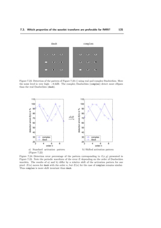
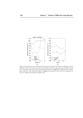
![7.2. Description of the algorithm 113
filters are bi-orthonormal, they are mostly chosen orthonormal in the literature,
i.e., ˜H(z) = H(z−1
) and ˜G(z) = G(z−1
); this is in particular the case for the
Daubechies filters [43]. For such filters, which are automatically half-band, there
remains only one tradeoff between the sharpness of the frequency cutoff and the
spatial localization. Because we want to optimize our detection scheme with respect
to orthonormal and bi-orthonormal transforms, we use as first choice the new class
of scaling functions and wavelets that provide this flexibility: the fractional splines
[145] (Section 4.2.1).
→ Complex wavelets. The discrete real wavelet transform is quite sensitive to a
shift of the input signal due to down-sampling. This effect is significantly reduced
when considering the coefficient magnitudes of the Complex Wavelet Transform
(CWT). An additional advantage of the CWT for 2 dimensions is that it offers six
angle-selective subbands rather than three in the case of real DWT. Furthermore,
the computational cost of the CWT is the same as two real DWT [118, 29].
→ Quincunx wavelets. The use of such wavelets is interesting because of some
advantages it offers over separable wavelets (e.g. fractional splines and Daubechies
wavelets):
i) The scale reduction of the separable scheme progresses by powers of 2. Quin-
cunx has a finer scale progression—by powers of
√
2—and can thus detect
more accurately very fine/capillary activation patterns or can better provide
the adequate iteration depth for noise reduction.
ii) The separable wavelets have a strong directionality. Activation patterns which
are expanded in horizontal or vertical directions are better detected than diag-
onal expanded patterns. Quincunx has the advantage of providing an analysis
that is more isotropic.
7.2.3 Activation detection by statistical testing on the wavelet coef-
ficients
Because of the noise present in the data, it is almost impossible to detect any activation
without resorting to statistical analysis. This analysis requires a model of noise [57];
here, we assume that IDτ (x, y) follows a spatial Gaussian distribution. Thanks to the
wavelet transform, simple statistics can be applied, which makes the analysis fast and
straightforward. Thus, a statistical testing on each coefficient of IWτ (x, y) will be applied
to determine whether it is activated or not (refer to Section 3.3.5). In the case of real
wavelets, a Student t-test is applied as described in Section 3.3.3. At this stage, all
non-significant wavelet coefficients are set to zero, keeping only those that have been
labeled as “activated”. This yields the W-estimated activation Iest,W(x, y) (WEA). An
example of Iest,W(x, y) for the data of Figure 7.1 is presented in Figure 7.5. In the](https://image.slidesharecdn.com/0eba55bf-42a7-4963-8f0c-60b852f024ac-160911124222/85/feilner0201-147-320.jpg)
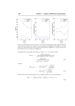
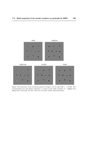
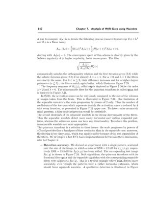
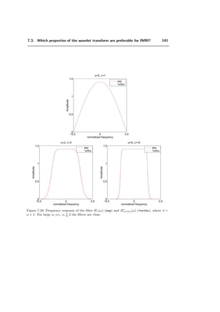
![118 Chapter 7. Analysis of fMRI Data using Wavelets
activated pixels:
E1 =
Card {(x, y) : I(x, y) = 0 and Iest(x, y) = 0}
Card(A)
(7.2)
• the number of missed detections, i.e., errors of type II (E2), relative to the number
of activated pixels:
E2 =
Card {(x, y) : I(x, y) = 0 and Iest(x, y) = 0}
Card(A)
Thus the relation (1−E1) is the percentage of pixels correctly detected as non-activated,
which determines the specificity. In theory, this value can be negative, but in practice,
negative values rarely occur. The relation (1 − E2) is the percentage of pixels which
were properly detected, and determines the sensitivity. The error types E1 and E2 are
illustrated in Figure 7.9. Our global error criterion to minimize is, by definition, the
total error, which is the sum of the two types of errors: E = E1 + E2. Note that
even though this quantity provides a fair control on the localization of the activation
zone, it cannot give clues on the amplitude mismatch. Obviously, the activation pattern
needs to be known to compute E. A related measure, first applied to the analysis of
(missed detections)
Error Type II (= E2)
(false detections)
Error Type I (= E1)
A
Iest
Ac
Figure 7.9: Example of a schematic detection of a quadratic pattern. The global error criterion
is defined as E = E1 + E2.
fMRI processing techniques by [34], is the Receiver Operator Characteristic (ROC). With
ROC, the relationship between the true-positive ratio (proportion of correctly detected
activations to all true activations) and the false-positive ratio (proportion of pixels that
were incorrectly recognized as active in all pixels without true activations) is measured,
depending on a parameter that controls the sensitivity of the detection procedure [129].
In our case this parameter would be the threshold in the wavelet t-domain (which we set
to the value that ensures less than 5% of false detections). Compared to the measures](https://image.slidesharecdn.com/0eba55bf-42a7-4963-8f0c-60b852f024ac-160911124222/85/feilner0201-152-320.jpg)
![7.3. Which properties of the wavelet transform are preferable for fMRI? 119
E1 and E2, the true-positive ratio is equal to (1 − E2) and the false-positive ratio is
proportional to E1. It is the denominator of the definition of these measures that makes
the difference: compare (7.2) with:
false positive ratio = E1
Card(A)
Card(Ac)
(7.3)
Thus, the ROC-curve, compared to our measures is:
ROC(γ) =
1 − E2(γ)
E1(γ) Card(A)
Card(Ac)
where γ ∈ [0%, 100%]. (7.4)
We believe that it is more reasonable to express the false detections (E1) relative to A,
rather than Ac
because then: (i) the quantity E1 and E2 are comparable (ii) E1 does
not depend on the image size and (iii) a larger activation zone is likely to cause more
false activations. In Figure 7.10 such a ROC curve is illustrated in terms of E1 and E2.
Minimizing E amounts to maximizing 1 − E, i.e., the distance between the ROC-curve
and the locus of random detection, which represents 1−E = 1−E2−E1 = 0. When the
curve lies below the locus of random detection, the minimal error is the minimal distance
of the ROC-curve to this diagonal. A field where these error measures are intensively
40%
1 − E = 0
E1
80%40%20%0%
0%
20%
1 − E
60%
80%
EER
1−E2
ROC
E1 = E2
Figure 7.10: Comparison of Receiver Operator Characteristic (ROC), the Equal Error Rate
(EER) and our error measure (E).
studied is biometrics, the field of automatic identity verification methods, such as voice,
face, eyes or fingerprint identification. They cope with the False Rejection Rate (FRR),
which is equal to our E2 and with False Acceptance Rate (FAR) which is equal to the
false positive ratio. In this field, the Equal Error Rate (EER), given by E1 = E2 on the
ROC-curve, is often used as a performance measure; see the position compared to the](https://image.slidesharecdn.com/0eba55bf-42a7-4963-8f0c-60b852f024ac-160911124222/85/feilner0201-153-320.jpg)
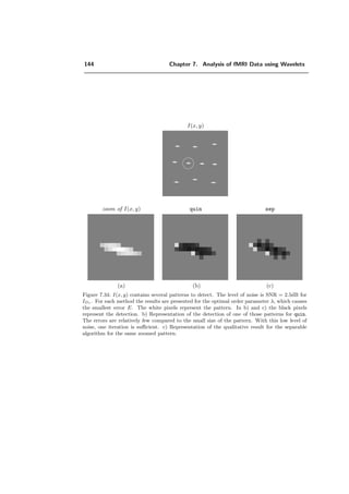
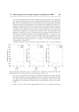
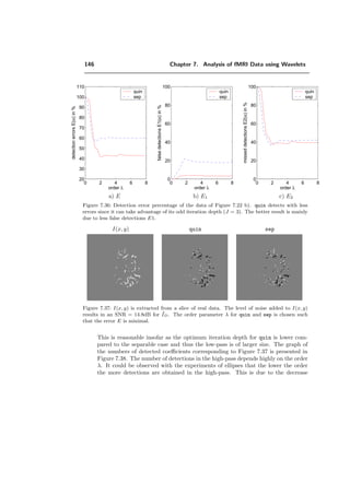
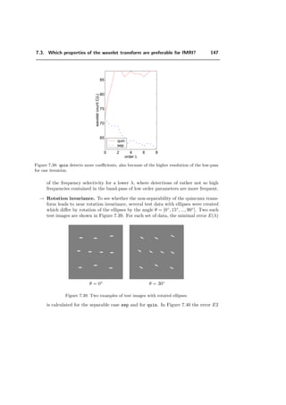
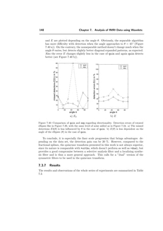
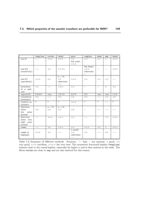
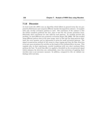
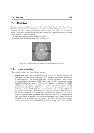
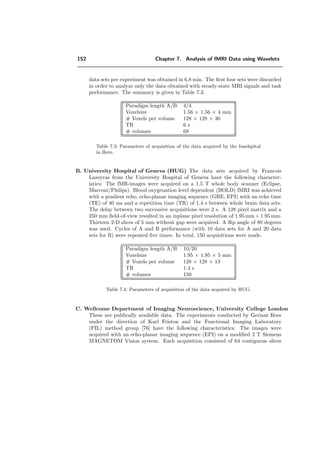
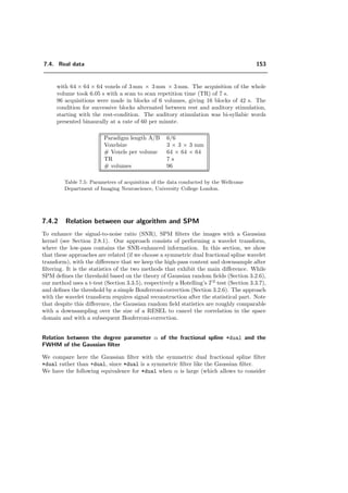

![7.3. Which properties of the wavelet transform are preferable for fMRI? 131
→ Translation invariance. Similarly to other real wavelets due to the down-
sampling operation, the fractional spline wavelets are not translation invariant.
In addition the causal fractional splines shift their center by α+1
2 .
→ Rotation invariance. Since the FSWT is a separable transform, it should not
exhibit any rotational invariance. However, the dual shows the best isotropy and
thus should yield the best rotation invariance.
To make a global choice over all FSWT, we propose to take +dual with α = 1.2 − 1.6
and an iteration step of 1 or 2, depending on the amount of noise. When the noise level
is very high, the method performs better by using only the low-pass. +bspline performs
well for the degree parameter α = 0.2 − 0.6 when low noise is present. It controls the
error of false detections strongly.
7.3.5 Complex wavelets
The structure of the complex wavelets is described in Section 4.4. We recall here that
the CWT has the advantage of being closer to shift invariance than its real counterpart
while keeping the computational cost low.
The frequency response of the real Daubechies and of the complex Daubechies with low-
pass and with high-pass filters are presented in Figure 7.20 for the order parameter n = 3
and n = 7. The filters are orthogonal and compactly supported (in the complex case
[−n, n + 1], n ∈ Z). In addition, the complex Daubechies filters are symmetric.
n = 3 n = 7
0 0.1 0.2 0.3 0.4 0.5
0
0.5
1
1.5
normalized frequency
0 0.1 0.2 0.3 0.4 0.5
0
0.5
1
1.5
normalized frequency
Figure 7.20: Example of frequency response of the low-pass (solid line) and high-pass (dashed
line) filters for the complex Daubechies wavelets (complex), which are the same for the real
Daubechies.
→ Shift invariance. Figure 7.21 illustrates that the complex filters are more shift
invariant than the real Daubechies filters. Each plot shows the energy of the 1D](https://image.slidesharecdn.com/0eba55bf-42a7-4963-8f0c-60b852f024ac-160911124222/85/feilner0201-165-320.jpg)
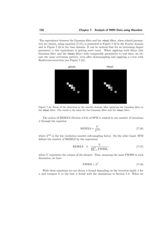
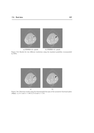
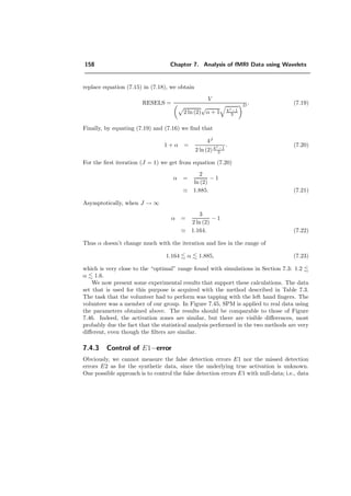
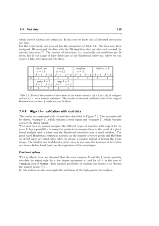
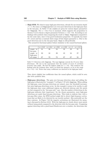
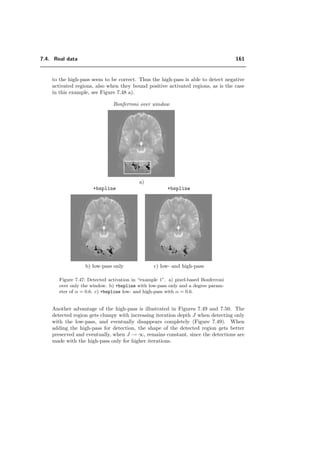
![138 Chapter 7. Analysis of fMRI Data using Wavelets
2 4 6 8
50
55
60
65
70
75
80
85
order n
count(n)
complex
daub
2 4 6 8
0
10
20
30
40
50
order n
falsedetectionsE1(n)
complex
daub
2 4 6 8
0
10
20
30
40
50
order n
misseddetectionsE2(n)
complex
daub
a) C b) E1 c) E2
Figure 7.27: Illustration of wavelet count C, E1 and E2 corresponding to the detection with the
same data like in Figure 7.26. count(α) is always higher for complex than for daub (a). For this
reason, the missed detections E2 are usually much smaller for complex (c). On the contrary the
false detections E1 are higher for complex (b).
orthogonal fractional spline filter Bα
∗ortho with α = λ − 1 as shown below:
Hλ(ω) =
√
2(2 + 2 cos ω)
λ
2
(2 + 2 cos ω)λ + (2 − 2 cosω)λ
=
√
2 cos ω
2
λ
cos ω
2
2λ
+ sin ω
2
2λ
(7.6)
whereas
Bα
∗ortho(ω) =
√
2
1 + e−jω
2
α+1
Aα(ω)
Aα(2ω)
=
√
2 cos
ω
2
α+1 Aα(ω)
Aα(2ω)
. (7.7)
Call that the autocorrelation filter A(ω) satisfies ([135]) the two-scale relation:
A(2ω) =
1
2
|Bα
∗ (ω)|2
A(ω) +
1
2
|Bα
∗ (ω + π)|2
A(ω + π).
(7.8)](https://image.slidesharecdn.com/0eba55bf-42a7-4963-8f0c-60b852f024ac-160911124222/85/feilner0201-172-320.jpg)
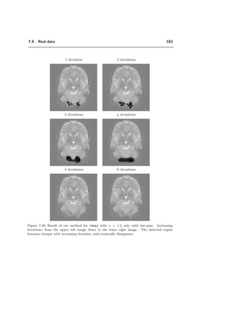
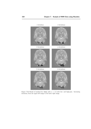
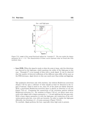
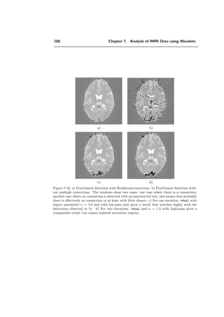
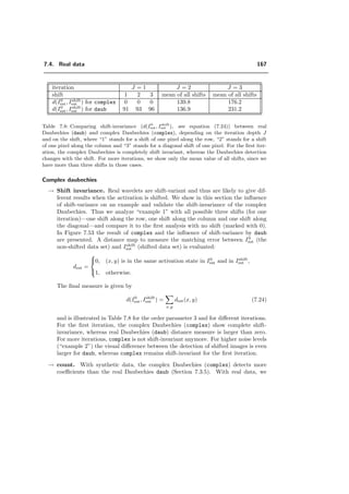
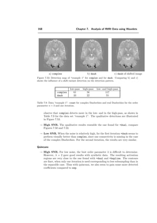
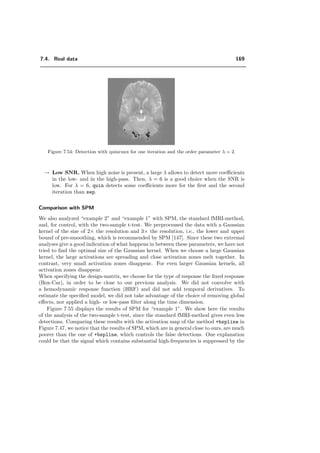
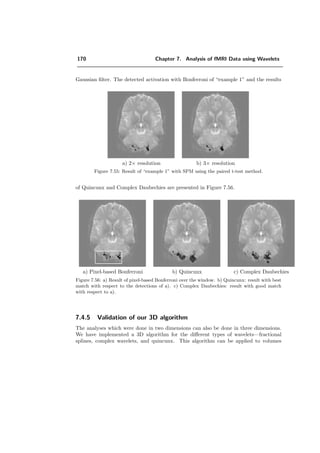
![7.3. Which properties of the wavelet transform are preferable for fMRI? 147
0 2 4 6 8
65
70
75
80
85
order λ
waveletcountC(λ)
quin
sep
Figure 7.38: quin detects more coefficients, also because of the higher resolution of the low-pass
for one iteration.
of the frequency selectivity for a lower λ, where detections of rather not so high
frequencies contained in the band-pass of low order parameters are more frequent.
→ Rotation invariance. To see whether the non-separability of the quincunx trans-
form leads to near rotation invariance, several test data with ellipses were created
which differ by rotation of the ellipses by the angle θ = [0◦
, 15◦
, ..., 90◦
]. Two such
test images are shown in Figure 7.39. For each set of data, the minimal error E(λ)
θ = 0◦
θ = 30◦
Figure 7.39: Two examples of test images with rotated ellipses.
is calculated for the separable case sep and for quin. In Figure 7.40 the error E2](https://image.slidesharecdn.com/0eba55bf-42a7-4963-8f0c-60b852f024ac-160911124222/85/feilner0201-181-320.jpg)
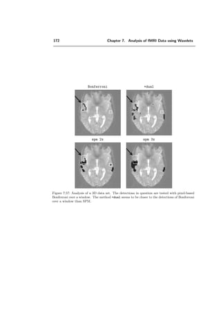

![150 Chapter 7. Analysis of fMRI Data using Wavelets
7.3.8 Discussion
A recent work [44] (2001) uses an algorithm which follows in general terms the one pro-
posed by Ruttimann and compares different wavelet decomposition schemes. A template
with only circular activation patterns is used. The conclusion of the authors is that
the Gabor transform performs the best, since it best fits the circular activation areas.
Obviously, their conclusions are only valid for such patterns. To carefully prevent this
problem, we used different non symmetric activation shapes [59] (2000). We also avoided
using different pattern sizes in the same image, since in this case the large patterns dom-
inate the error measure and no information is given for small activation patterns. The
signal reconstruction method of [44] seems to cause ringing and thus the false detection
errors get more prominent for wavelets as the length of the synthesis filters increase. This
explains why, in their experiments, wavelet transforms with very short synthesis filters
perform the best. To avoid this effect we applied a threshold on the reconstructed signal
which enhances the detection rate substantially, since this restriction of applying short
wavelets only is not necessary anymore. In addition, compared to [44], we validate our
findings with real data.](https://image.slidesharecdn.com/0eba55bf-42a7-4963-8f0c-60b852f024ac-160911124222/85/feilner0201-184-320.jpg)
![7.4. Real data 151
7.4 Real data
In this section, we validate the results of the synthetic data (Section 7.3) with real data.
For this purpose, we considered several real data sets from different subjects and for
different tasks. For example, tapping with the left or right hand fingers was one of these
tasks. Other tasks were moving the shoulder, looking at a light source switching on and
off or listening to bi-syllabic words.
The orientation of the images is shown in Figure 7.41.
We also compare our method with SPM (Section 2.8).
Left
Posterior
Anterior
Right
Figure 7.41: Orientation of the brain in the images along this section.
7.4.1 Image acquisition
We obtained the data sets from different sources.
A. Inselspital of Bern The data sets acquired by Arto Nirkko from the Inselspital of
Bern have the following characteristics ([105]): The fMR-images were acquired on
a standard clinical 1.5 T whole body scanner (Siemens Magnetom Vision). Blood
Oxygenation Level Dependent (BOLD) (see Section 2.3) fMRI was achieved with an
Echo-Planar Imaging sequence (EPI) (see Section 2.2.3) with an Echo Time (TE)
of 62 ms and a Repetition Time (TR) of 6 s between whole brain data sets. A 128
pixel matrix and a 200 mm field-of-view resulted in an inplane pixel resolution of
1.56 mm×1.56 mm. Thirty 2-D slices of 5 mm thickness and 4 mm spacing between
slice centers were acquired. Since distortions in the phase-encoding direction cannot
be avoided completely, the phase-encoding direction was selected in the antero-
posterior direction, thus preserving brain symmetry. In total, 68 measurements
were acquired per experiment. The volunteer had to alternate between activation
(A) and rest (B) periods according to auditory cues. Cycles of A and B performance
(each with four data sets, equaling 24 s) were repeated eight times. The total of 68](https://image.slidesharecdn.com/0eba55bf-42a7-4963-8f0c-60b852f024ac-160911124222/85/feilner0201-185-320.jpg)
![152 Chapter 7. Analysis of fMRI Data using Wavelets
data sets per experiment was obtained in 6.8 min. The first four sets were discarded
in order to analyze only the data obtained with steady-state MRI signals and task
performance. The summary is given in Table 7.3.
Paradigm length A/B 4/4
Voxelsize 1.56 × 1.56 × 4 mm
# Voxels per volume 128 × 128 × 30
TR 6 s
# volumes 68
Table 7.3: Parameters of acquisition of the data acquired by the Inselspital
in Bern.
B. University Hospital of Geneva (HUG) The data sets acquired by Francois
Lazeyras from the University Hospital of Geneva have the following character-
istics: The fMR-images were acquired on a 1.5 T whole body scanner (Eclipse,
Marconi/Philips). Blood oxygenation level dependent (BOLD) fMRI was achieved
with a gradient echo, echo-planar imaging sequence (GRE, EPI) with an echo time
(TE) of 40 ms and a repetition time (TR) of 1.4 s between whole brain data sets.
The delay between two successive acquisitions were 2 s. A 128 pixel matrix and a
250 mm field-of-view resulted in an inplane pixel resolution of 1.95 mm × 1.95 mm.
Thirteen 2-D slices of 5 mm without gap were acquired. A flip angle of 80 degrees
was used. Cycles of A and B performance (with 10 data sets for A and 20 data
sets for B) were repeated five times. In total, 150 acquisitions were made.
Paradigm length A/B 10/20
Voxelsize 1.95 × 1.95 × 5 mm
# Voxels per volume 128 × 128 × 13
TR 1.4 s
# volumes 150
Table 7.4: Parameters of acquisition of the data acquired by HUG.
C. Wellcome Department of Imaging Neuroscience, University College London
These are publically available data. The experiments conducted by Geriant Rees
under the direction of Karl Friston and the Functional Imaging Laboratory
(FIL) method group [76] have the following characteristics: The images were
acquired with an echo-planar imaging sequence (EPI) on a modified 2 T Siemens
MAGNETOM Vision system. Each acquisition consisted of 64 contiguous slices](https://image.slidesharecdn.com/0eba55bf-42a7-4963-8f0c-60b852f024ac-160911124222/85/feilner0201-186-320.jpg)


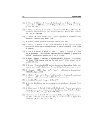
![7.4. Real data 169
Figure 7.54: Detection with quincunx for one iteration and the order parameter λ = 2.
→ Low SNR. When high noise is present, a large λ allows to detect more coefficients
in the low- and in the high-pass. Then, λ = 6 is a good choice when the SNR is
low. For λ = 6, quin detects some coefficients more for the first and the second
iteration than sep.
Comparison with SPM
We also analyzed “example 2” and “example 1” with SPM, the standard fMRI-method,
and, for control, with the two-sample t-test. We preprocessed the data with a Gaussian
kernel of the size of 2× the resolution and 3× the resolution, i.e., the lower and upper
bound of pre-smoothing, which is recommended by SPM [147]. Since these two extremal
analyses give a good indication of what happens in between these parameters, we have not
tried to find the optimal size of the Gaussian kernel. When we choose a large Gaussian
kernel, the large activations are spreading and close activation zones melt together. In
contrast, very small activation zones disappear. For even larger Gaussian kernels, all
activation zones disappear.
When specifying the design-matrix, we choose for the type of response the fixed response
(Box-Car), in order to be close to our previous analysis. We did not convolve with
a hemodynamic response function (HRF) and did not add temporal derivatives. To
estimate the specified model, we did not take advantage of the choice of removing global
effects, nor applied a high- or low-pass filter along the time dimension.
Figure 7.55 displays the results of SPM for “example 1”. We show here the results
of the analysis of the two-sample t-test, since the standard fMRI-method gives even less
detections. Comparing these results with the activation map of the method +bspline in
Figure 7.47, we notice that the results of SPM, which are in general close to ours, are much
poorer than the one of +bspline, which controls the false detections. One explanation
could be that the signal which contains substantial high-frequencies is suppressed by the](https://image.slidesharecdn.com/0eba55bf-42a7-4963-8f0c-60b852f024ac-160911124222/85/feilner0201-203-320.jpg)