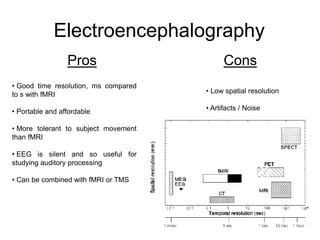
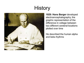
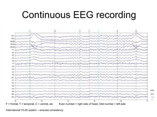
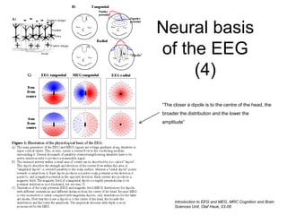
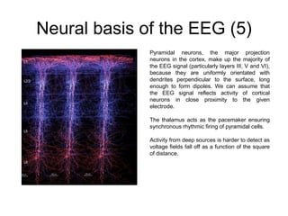
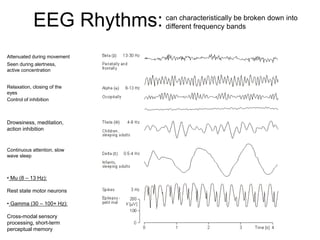
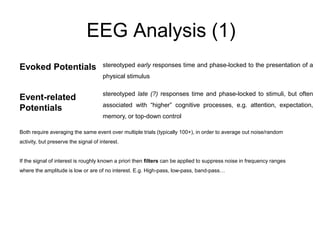
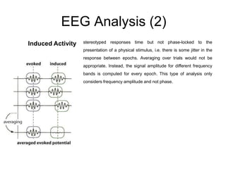
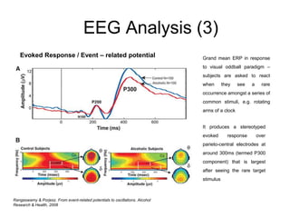
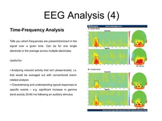
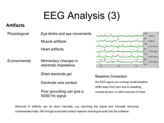
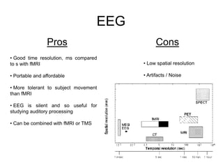
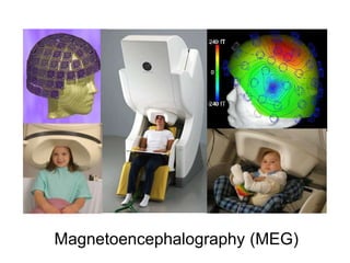
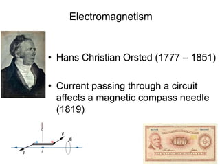
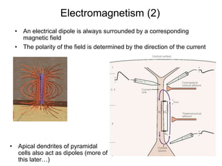
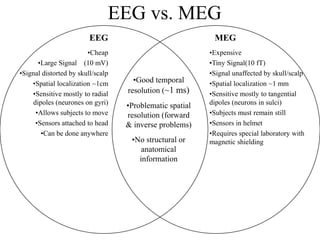
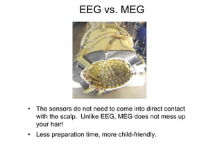
Methods for Dummies
15.02.2012
Marcos Economides
Spas Getov
Basis of the EEG/MEG signal
Electroencephalography
Pros Cons
• Good time resolution, ms compared
to s with fMRI
• Portable and affordable
• More tolerant to subject movement
than fMRI
• EEG is silent and so useful for
studying auditory processing
• Can be combined with fMRI or TMS
• Low spatial resolution
• Artifacts / Noise
• Richard Caton (1842-1926) from Liverpool published findings about
electrical phenomena of the exposed cerebral hemispheres of rabbits and
monkeys in the British Medical Journal in 1875.
• In 1890 Adolf Beck published findings of spontaneous electrical activity and
rhythmic oscillations in response to light in the brains of rabbits and dogs.
• In 1912 Vladimir Vladimirovich Pravdich-Neminsky published the first animal
EEG study described evoked potential in the mammalian brain.
• In 1914 Napoleon Cybulski and Jelenska-Macieszyna photographed EEG
recordings of experimentally induced seizures.
History
History
1929: Hans Berger developed
electroencephalography, the
graphic representation of the
difference in voltage between
two different cerebral locations
plotted over time
He described the human alpha
and beta rhythms
Continuous EEG recording
F = frontal, T = temporal, C = central, etc Even number = right side of head, Odd number = left side
International 10-20 system – ensures consistency
Digital vs. Analogue
• Conventional analogue instruments consist of an amplifier, a galvanometer (a coil of
wire inside a magnetic field) and a writing device. The output signal from the amplifier
passes through the wire causing the coil to oscillate, and a pen mounted on the
galvanometer moves up and down in sync with the coil, drawing traces onto paper.
• Digital EEG systems convert the waveform into a series of numerical values, a
process known as Analogue-to-Digital conversion. The rate at which waveform data
is sampled is known as the sampling rate, and as a rule should be at least 2.5 times
greater than the highest frequency of interest. Most digital EEG systems will sample
at 240Hz.
• The accuracy of digital EEG waveforms can be affected by sampling skew – a small
time lag that occurs when each channel is sampled sequentially. This can be reduced
using burst mode – reduced the time lag between successive channel sampling.
• Be aware of the relationship between sampling rate, screen resolution and the EEG
display. If there are more data samples than there are pixels then this will have the
effect of reducing the sampling rate and the data displayed will appear incomplete.
However, most modern digital EEG systems will draw two data samples per screen
pixel.
EEG Acquisition
Electrodes: Usually made of silver (or
stainless steel) – active electrodes placed
on the scalp using a conductive gel or paste.
Signal-to-noise ratio (impedance) reduced
by light abrasion. Can have 32, 64,128, 256
electrodes. More electrodes = richer data
set. Reference electrodes (arbitrarily chosen
“zero level”, analogous to sea level when
measuring mountain heights) commonly
placed on the midline, ear lobes, nose, etc.
Amplification: one pair of electrodes
make up one channel on the differential
amplifier, i.e. there is one amplifier per pair
of electrodes. The amplifier amplifies the
difference in voltage between these two
electrodes, or signals (usually between 1000
and 100 000 times). This is usually the
difference between an active electrode and
the designated reference electrode.
EEG records differences in voltage: the way in which the signal is viewed can be
set up in a variety of ways called montages
Bipolar montage: Each waveform in the EEG represents the difference in voltage between two adjacent
electrodes, e.g. ‘F3-C3’ represents the difference in voltage between channel F3 and neighbouring channel C3. This
is repeated across the whole scalp through the entire array of electrodes.
Reference montage: Each waveform in the EEG represents the difference in voltage between a specific
active electrode and a designated reference electrode. There is no standard position for the reference, but usually a
midline electrode is chosen so as not to bias the signal in any one hemisphere. Other popular reference signals
include an average signal from electrodes placed on each ear lobe or mastoid.
Average Reference montage: Activity from all electrodes is measured, summed and then averaged.
The resulting signal is then used as a reference electrode and acts as input 2 of the amplifier. The use can specify
which electrodes are to be included in this calculation.
Laplacian montage: Similar to average reference, but this time the common reference is a weighted
average of all the electrodes, and each channel is the difference between the given electrode and this common
reference.
Montages (continued)
• In digital EEG setups, the data is usually stored onto computer memory in reference
mode, regardless of the montage used to display the data when it is being recorded.
• This means that “remontaging”, i.e. changing the montage either ‘on-line’ or ‘off-line’,
can be done via a simple subtraction which cancels out the common reference.
F3 – Reference F4 – Reference
-
= F3 – F4
E.g.
What does the EEG record?
Volume conduction
Ions are constantly flowing in and out of neurons to
maintain resting potential and propogate action
potentials. Movement of like-charged ions out of
numerous neighbouring neurons can create waves of
electrical charge, which can push or pull electrons on
scalp electrodes, creating voltage differences.
In summary, the EEG signal represents the deflection of
electrons on the scalp electrodes, caused by cortical
“dipoles” (the summed activity within a specific area of
cortex that creates a current flow).
Neural basis of the EEG (1)
Action Potentials
Rapid, transient, all-or-none nerve impulses
that flow from the body to the axon terminal of
a neuron.
They are generally too short in duration (a few
ms) and to “deep” to contribute significantly to
the EGG signal.
In addition they create 2 dipoles = quadrupole
Finally, synchronous firing is unlikely
preventing the summation of potentials
Neural basis of the EEG (2)
Post-synaptic potentials Scalp EEG is a summation of non-
propogating dendritic and somatic post-
synaptic potentials which arise relatively
slower than action potentials (approx 10ms).
EPSPs – Excitatory Post Synaptic Potentials
IPSPs – Inhibitory Post Synaptic Potentials
Post synaptic potentials summate spatially
and temporally – A single pyramidal cell may
have more than 104 synapses distributed
over its soma and dendritic surface.
Neural basis of the EEG (3)
When an EPSP is generated in the dendrites of a
neuron, Na+ flow inside the neuron’s cytoplasm creating
a current sink.
The current completes a loop creating a dipole further
away from the excitatory input (where Na+ flows outside
the cell as passive return current), which can be
recorded as a positive voltage difference by an
extracellular electrode.
Large numbers of vertically oriented, neighbouring
pyramidal neurons create these field potentials.
Thus, EEG detects summed synchronous activity
(PSPs) from many thousands of apical dendrites of
neighbouring pyramidal cells (mainly).
+
-
Synapse
Dendrites
“It takes a combined synchronous electrical activity of approximately
108 neurons in a minimal cortical area of 6cm2 to create visible
EEG”… Olejniczak, J. Clinical Neurophysiology, 2006.
Introduction to EEG and MEG, MRC Cognition and Brain
Sciences Unit, Olaf Hauk, 03-08
Neural basis
of the EEG
(4)
“The closer a dipole is to the centre of the head, the
broader the distribution and the lower the
amplitude”
Neural basis of the EEG (5)
Pyramidal neurons, the major projection
neurons in the cortex, make up the majority of
the EEG signal (particularly layers III, V and VI),
because they are uniformly orientated with
dendrites perpendicular to the surface, long
enough to form dipoles. We can assume that
the EEG signal reflects activity of cortical
neurons in close proximity to the given
electrode.
The thalamus acts as the pacemaker ensuring
synchronous rhythmic firing of pyramidal cells.
Activity from deep sources is harder to detect as
voltage fields fall off as a function of the square
of distance.
EEG Rhythms:
Attenuated during movement
Seen during alertness,
active concentration
Relaxation, closing of the
eyes
Control of inhibition
Drowsiness, meditation,
action inhibition
Continuous attention, slow
wave sleep
• Mu (8 – 13 Hz):
Rest state motor neurons
• Gamma (30 – 100+ Hz):
Cross-modal sensory
processing, short-term
perceptual memory
can characteristically be broken down into
different frequency bands
EEG Analysis (1)
stereotyped early responses time and phase-locked to the presentation of a
physical stimulus
stereotyped late (?) responses time and phase-locked to stimuli, but often
associated with “higher” cognitive processes, e.g. attention, expectation,
memory, or top-down control
Evoked Potentials
Event-related
Potentials
Both require averaging the same event over multiple trials (typically 100+), in order to average out noise/random
activity, but preserve the signal of interest.
If the signal of interest is roughly known a priori then filters can be applied to suppress noise in frequency ranges
where the amplitude is low or are of no interest. E.g. High-pass, low-pass, band-pass…
EEG Analysis (2)
Induced Activity stereotyped responses time but not phase-locked to the
presentation of a physical stimulus, i.e. there is some jitter in the
response between epochs. Averaging over trials would not be
appropriate. Instead, the signal amplitude for different frequency
bands is computed for every epoch. This type of analysis only
considers frequency amplitude and not phase.
EEG Analysis (3)
Evoked Response / Event – related potential Grand mean ERP in response
to visual oddball paradigm –
subjects are asked to react
when they see a rare
occurrence amongst a series of
common stimuli, e.g. rotating
arms of a clock
It produces a stereotyped
evoked response over
parieto-central electrodes at
around 300ms (termed P300
component) that is largest
after seeing the rare target
stimulus
Rangaswamy & Porjesz. From event-related potentials to oscillations. Alcohol
Research & Health, 2008
EEG Analysis (4)
Time-Frequency Analysis
Tells you which frequencies are present/dominant in the
signal over a given time. Can be for one single
electrode or the average across multiple electrodes.
Useful for:
• Analysing induced activity that isn’t phase-locked, i.e.
that would be averaged out with conventional event-
related analysis
• Characterising and understanding typical responses to
specific events – e.g. significant increase in gamma
band activity 20-60 ms following an auditory stimulus
EEG Analysis (3)
Artifacts
Eye blinks and eye movements
Muscle artifacts
Heart artifacts
Physiological
Environmental Momentary changes in
electrode impedance
Dried electrode gel
Electrode wire contact
Poor grounding can give a
50/60 Hz signal
Removal of artifacts can be done manually, e.g. epoching the signal and manually removing
contaminated trials; OR through automated artifact rejection techniques build into the software.
Baseline Correction
the EEG signal can undergo small baseline
shifts away from zero due to sweating,
muscle tension, or other sources of noise.
EEG
Pros Cons
• Good time resolution, ms compared
to s with fMRI
• Portable and affordable
• More tolerant to subject movement
than fMRI
• EEG is silent and so useful for
studying auditory processing
• Can be combined with fMRI or TMS
• Low spatial resolution
• Artifacts / Noise
Magnetoencephalography (MEG)
• Hans Christian Orsted (1777 – 1851)
• Current passing through a circuit
affects a magnetic compass needle
(1819)
Electromagnetism
• An electrical dipole is always surrounded by a corresponding
magnetic field
• The polarity of the field is determined by the direction of the current
Electromagnetism (2)
• Apical dendrites of pyramidal
cells also act as dipoles (more of
this later…)
• The magnetic fields generated by the
brain are minute: 100 million times
weaker than the earth’s magnetic field,
one million times weaker than the
magnetic fields generated by the urban
environment.
• By way of contrast, MRI scanners
generate a magnetic field of between 3
to 3.5 tesla.
Biomagnetic Fields
But…
• First recording of biomagnetic field generated by the human hart (Gerhard
Baule and Richard Mcfee, 1963)
• Two copper pick-up coils twisted round a ferrite core with 2 million turns.
• The two coils were connected in opposite directions so as to cancel out the
background fluctuations. Never the less, they had to conduct their experiment
in the middle of a field because the signal was still very noisy.
• A group working in the Soviet Union (Safonev et al, 1967) produced similar
results but in a shielded room: reduced background noise by a factor of 10.
• Thermal noise was limiting in the use of copper.
Early Recordings of Biomagnetic Fields
Recording Biomagnetic Fields From the Brain
• David Cohen and
colleagues make
measurements using a
copper induction coil in a
magnetically shielded room
in University of Illinois.
• Measurements were too
noisy for useful analysis
1968
Two key problems:
1. Sensors sensitive enough to record tiny changes in magnetic flux
2. Eliminate ‘noise’ from other environmental fluctuations in flux
- When cooled to -269C, solid mercury
suddenly lost all resistance to the flow of
electric current (Heike Onnes, 1911) .
“Superconductivity”
-Later found in other materials, such as tin
and metal alloys.
- When two superconducting materials are
separated by a thin insulating layer a
‘tunnel effect’ is produced which enables
the flow of electrons - even in the absence
of any external voltage. This is a
Josephson Junction (Brian Josephson
1962).
Superconductivity
Recording a Weak Signal: SQUIDs
Create a superconducting loop and
measure changes in interference of
quantum-mechanical electron waves
circulating in this loop as magnetic flux
in loop changes
Invented at Ford Research Labs in
1964/1965 by Jaklevic, Lambe, Silver,
Mercerau and Zimmerman
Two types: DC and RF SQUIDs. RF
squids generally used to make
measurements of biomagnetism (less
sensitive but much cheaper).
Niobium or lead alloy cooled to near
absolute zero with liquid helium
Can measure magnetic fields as small
as 1 femtotesla (10-15)
• David Cohen, now at
MIT, used one of the first
SQUIDs to record a
cleaner MEG signal.
• By now they had
designed a better
magnetically sheilded
room.
• Used one SQUID only,
which was moved
around to different
positions
1972
Recording Biomagnetic Fields From the Brain
Since 1980s – multiple SQUIDs arranged
in arrays to allow measurement over the
whole scalp surface
The helmet-shaped dewar of current
systems typically contains around 300
sensors (connected to SQUIDs) and
contains liquid helium to keep the sensors
cooled enough to superconduct.
Carefully designed and constructed
magnetically shielded rooms. Different
metals used to shield different frequencies
of magnetic interference.
Modern MEG
Minimising Noise
Flux Transformers
Convert changes in magnetic flux to
changes in current.
Magnetometers: pick up environmental
‘noise’
Gradiometers: two or more coils –
magnetic interferance from distant
sources uniform across them while
interferance from close by isn’t
Changes in output from gradiometer to
SQUID are caused mainly by changes
in flux close-by (in subject’s brain).
Only a small percentage of the external
noise arrives at the SQUID.
Neural Basis of the MEG Signal
Magnetic fields are produced by same electrical changes recorded by EEG
Again, the main source is post-synaptic currents flowing across pyramidal
neurones… as previously described
However, there are some key differences:
1. Magnetic field is perpendicular to current
• If the current is running parallel to the scalp the magnetic field exits the head from
one side of the dipole and re-enters on the other side and so can be measured.
• But if the current is perpendicular to the scalp the magnetic field does not leave
the scalp and cannot be measured.
• MEG is more sensitive to activity of
pyramidal cells in the walls of the sulci.
• MEG registers no information from radially
aligned axons (unlike EEG)
• MEG signal decays more quickly with
distance (in proportion to distance2) so
problems recording deep (subcortical)
areas
2. Differential sensitivity by brain region
http://www.scholarpedia.org/article/MEG
Bone is transparent to
magnetism and magnetic fields
are not smeared by the
resistance of the skull.
Accurate reconstruction of the
neuronal activity that produced
the external magnetic fields
therefore requires simpler
models than with EEG
3. MEG signal is less distorted by skull/scalp
anatomy
Differences discussed in last slide mean that we can make stronger
inferences about the origin of the signals in MEG.
4. Different problems of source localisation
The Forward and Inverse Problems
1. Forward modelling generates
expected signal
2. Compare model to actual
recorded signal
3. Use difference between the
two to work backwards and
refine understanding of
where signal comes from
Forward Modelling:
1. Dipolar source models – can explain many configurations of electrical
current caused by groups of neurones and measured at ~ 2cm
2. Volume conductor models – modelling effects of cranial anatomy (simpler
for MEG).
The Inverse Problem
A given magnetic field recorded outside head could have been created by an enormous
number of possible electrical current distributions
→ Theoretically ill-posed as there are many possible solutions
Brookes et al 2010 (http://www.scholarpedia.org/article/MEG)
Source localisation models require
assumptions about brain physiology to
make the problem soluble
Many algorithms of source
reconstruction exist. This will be
covered in a future talk…
Dipole Fitting
Minimum norm approaches
Beamforming
MEG: Overview
http://web.mit.edu/kitmitmeg/whatis.html
Advantages/Disadvantages of MEG
http://web.mit.edu/kitmitmeg/whatis.html
EEG vs. MEG
•Good temporal
resolution (~1 ms)
•Problematic spatial
resolution (forward
& inverse problems)
•No structural or
anatomical
information
•Cheap
•Large Signal (10 mV)
•Signal distorted by skull/scalp
•Spatial localization ~1cm
•Sensitive mostly to radial
dipoles (neurones on gyri)
•Allows subjects to move
•Sensors attached to head
•Can be done anywhere
•Expensive
•Tiny Signal(10 fT)
•Signal unaffected by skull/scalp
•Spatial localization ~1 mm
•Sensitive mostly to tangential
dipoles (neurons in sulci)
•Subjects must remain still
•Sensors in helmet
•Requires special laboratory with
magnetic shielding
EEG MEG
• The sensors do not need to come into direct contact
with the scalp. Unlike EEG, MEG does not mess up
your hair!
• Less preparation time, more child-friendly.
EEG vs. MEG
MEG/EEG and Other Experimental
Approaches
ADVANTAGES OF M/EEG
• Non-invasive (records electromagnetic activity, does not modify it).
• More direct measure of neuronal function than metabolism-dependent
measures like BOLD signal in fMRI
• Can be used with adults, children, clinical population.
• High temporal resolution (up to 1 millisecond or less, around 1000x
better than fMRI) => ERPs study dynamic aspects
of cognition.
• Allow quiet environments.
• Subjects can perform tasks sitting up- more natural
than in MRI scanner
DISADVANTAGES OF M/EEG
• Problematic source localisation (forward & inverse
problems)
• Limited spatial resolution (especially EEG)
• Anatomical information not provided
Multimodal Imaging
http://www.neuroscience.cam.ac.uk/directory/profile.php?RikHenson
References/suggested reading
• Andro,W. and Nowak, H, (eds) (2007) Magnetism in Medicine. Wiley - VCN
• Handy, T. C. (2005). Event-related potentials. A methods handbook. Cambridge, MA: The MIT
Press.
• Luck, S. J. (2005). An introduction to the event-related potential technique. Cambridge,
Massachussets: The MIT Press
• Rugg, M. D., & Coles, M. G. H. (1995). Electrophysiology of mind: Event-related brain potentials and
cognition. New York, NY: Oxford University Press.
• Hamalainen, M., Hari, R., Ilmoniemi, J., Knuutila, J. & Lounasmaa, O.V. (1993). MEG: Theory,
Instrumentation and Applications to Noninvasive Studies of the Working Human Brain. Rev. Mod.
Phys. Vol. 65, No. 2, pp 413-497.
• Olejnickzac, P., (2006). Neurophysiologic basis of EEG. Journal of Clinical Neurophysiology, 23,
186-189.
• Silver, A.H. (2006). How the SQUID was born. Superconductor Science and Technology. Vol.19,
Issue 5 , pp173-178.
• Sylvain Baillet, John C. Mosher & Richard M. Leahy (2001). Electromagnetic Brain Mapping. IEEE
Signal Processing Magazine. Vol.18, No 6, pp 14-30.
• Basic MEG info:
• http://www1.aston.ac.uk/lhs/research/facilities/meg/introduction/
• http://web.mit.edu/kitmitmeg/whatis.html
• http://www.nmr.mgh.harvard.edu/martinos/research/technologiesMEG.php
• http://www.scholarpedia.org/article/MEG
References/suggested reading - EEG
• Speckmann & Elger. Introduction to the Neurophysiological Basis of the EEG and DC Potentials.
2005
• Williams & Wilkins. Electroencephalography: basic principles, clinical applications, and related fields.
15-26, 1993
• Introduction to EEG and MEG, MRC Cognition and Brain Sciences Unit, Olaf Hauk, 03-08
• Olejniczak, J. Clinical Neurophysiology, 2006
• Davidson, RJ, Jackson, DC, Larson, CL. Human electroencephalography. In: Cacioppo, JT,
Tassinary, LG, Bernston, GG, editors.
• Nunez, PL. Electric fields of the brain. 1st ed. New York, Oxford University Press, 1981.
• Introduction to quantitative EEG and neurofeedback. Evans, James R. (Ed);Abarbanel, Andrew (Ed)
San Diego, CA, US: Academic Press. (1999). xxi 406 pp.
• Goldman et al. Acquiring simultaneous EEG and functional MRI. Clinical Neurophysiology, 2000
• Handy, T.C. (2004) Event-Related Potentials: A Methods Handbook. MIT Press.
• Engel AK, Fries P, Singer W. (2001) Dynamic predictions: oscillations and synchrony in top-down
processing. Nature Reviews Neuroscience. 2(10):704-16.
• Lachaux JP, Rodriguez E, Martinerie J, Varela FJ. (1999) Measuring phase synchrony in brain
signals. Human Brain Mapping. 8(4):194-208.
• http://www.ebme.co.uk/arts/eegintro/index.htm
• http://psyphz.psych.wisc.edu/~greischar/BIW12-11-02/EEGintro.htm
• http://www.psych.nmsu.edu/~jkroger/lab/EEG_Introduction.html
EP vs. ERP / ERF
• evoked potential
– short latencies (< 100ms)
– small amplitudes (< 1μV)
– sensory processes
• event related potential / field
– longer latencies (100 – 600ms),
– higher amplitudes (10 – 100μV)
– higher cognitive processes

Basics of EEG

  • 1.
    Methods for Dummies 15.02.2012 MarcosEconomides Spas Getov Basis of the EEG/MEG signal
  • 2.
    Electroencephalography Pros Cons • Goodtime resolution, ms compared to s with fMRI • Portable and affordable • More tolerant to subject movement than fMRI • EEG is silent and so useful for studying auditory processing • Can be combined with fMRI or TMS • Low spatial resolution • Artifacts / Noise
  • 3.
    • Richard Caton(1842-1926) from Liverpool published findings about electrical phenomena of the exposed cerebral hemispheres of rabbits and monkeys in the British Medical Journal in 1875. • In 1890 Adolf Beck published findings of spontaneous electrical activity and rhythmic oscillations in response to light in the brains of rabbits and dogs. • In 1912 Vladimir Vladimirovich Pravdich-Neminsky published the first animal EEG study described evoked potential in the mammalian brain. • In 1914 Napoleon Cybulski and Jelenska-Macieszyna photographed EEG recordings of experimentally induced seizures. History
  • 4.
    History 1929: Hans Bergerdeveloped electroencephalography, the graphic representation of the difference in voltage between two different cerebral locations plotted over time He described the human alpha and beta rhythms
  • 5.
    Continuous EEG recording F= frontal, T = temporal, C = central, etc Even number = right side of head, Odd number = left side International 10-20 system – ensures consistency
  • 6.
    Digital vs. Analogue •Conventional analogue instruments consist of an amplifier, a galvanometer (a coil of wire inside a magnetic field) and a writing device. The output signal from the amplifier passes through the wire causing the coil to oscillate, and a pen mounted on the galvanometer moves up and down in sync with the coil, drawing traces onto paper. • Digital EEG systems convert the waveform into a series of numerical values, a process known as Analogue-to-Digital conversion. The rate at which waveform data is sampled is known as the sampling rate, and as a rule should be at least 2.5 times greater than the highest frequency of interest. Most digital EEG systems will sample at 240Hz. • The accuracy of digital EEG waveforms can be affected by sampling skew – a small time lag that occurs when each channel is sampled sequentially. This can be reduced using burst mode – reduced the time lag between successive channel sampling. • Be aware of the relationship between sampling rate, screen resolution and the EEG display. If there are more data samples than there are pixels then this will have the effect of reducing the sampling rate and the data displayed will appear incomplete. However, most modern digital EEG systems will draw two data samples per screen pixel.
  • 7.
    EEG Acquisition Electrodes: Usuallymade of silver (or stainless steel) – active electrodes placed on the scalp using a conductive gel or paste. Signal-to-noise ratio (impedance) reduced by light abrasion. Can have 32, 64,128, 256 electrodes. More electrodes = richer data set. Reference electrodes (arbitrarily chosen “zero level”, analogous to sea level when measuring mountain heights) commonly placed on the midline, ear lobes, nose, etc. Amplification: one pair of electrodes make up one channel on the differential amplifier, i.e. there is one amplifier per pair of electrodes. The amplifier amplifies the difference in voltage between these two electrodes, or signals (usually between 1000 and 100 000 times). This is usually the difference between an active electrode and the designated reference electrode.
  • 8.
    EEG records differencesin voltage: the way in which the signal is viewed can be set up in a variety of ways called montages Bipolar montage: Each waveform in the EEG represents the difference in voltage between two adjacent electrodes, e.g. ‘F3-C3’ represents the difference in voltage between channel F3 and neighbouring channel C3. This is repeated across the whole scalp through the entire array of electrodes. Reference montage: Each waveform in the EEG represents the difference in voltage between a specific active electrode and a designated reference electrode. There is no standard position for the reference, but usually a midline electrode is chosen so as not to bias the signal in any one hemisphere. Other popular reference signals include an average signal from electrodes placed on each ear lobe or mastoid. Average Reference montage: Activity from all electrodes is measured, summed and then averaged. The resulting signal is then used as a reference electrode and acts as input 2 of the amplifier. The use can specify which electrodes are to be included in this calculation. Laplacian montage: Similar to average reference, but this time the common reference is a weighted average of all the electrodes, and each channel is the difference between the given electrode and this common reference.
  • 9.
    Montages (continued) • Indigital EEG setups, the data is usually stored onto computer memory in reference mode, regardless of the montage used to display the data when it is being recorded. • This means that “remontaging”, i.e. changing the montage either ‘on-line’ or ‘off-line’, can be done via a simple subtraction which cancels out the common reference. F3 – Reference F4 – Reference - = F3 – F4 E.g.
  • 10.
    What does theEEG record? Volume conduction Ions are constantly flowing in and out of neurons to maintain resting potential and propogate action potentials. Movement of like-charged ions out of numerous neighbouring neurons can create waves of electrical charge, which can push or pull electrons on scalp electrodes, creating voltage differences. In summary, the EEG signal represents the deflection of electrons on the scalp electrodes, caused by cortical “dipoles” (the summed activity within a specific area of cortex that creates a current flow).
  • 11.
    Neural basis ofthe EEG (1) Action Potentials Rapid, transient, all-or-none nerve impulses that flow from the body to the axon terminal of a neuron. They are generally too short in duration (a few ms) and to “deep” to contribute significantly to the EGG signal. In addition they create 2 dipoles = quadrupole Finally, synchronous firing is unlikely preventing the summation of potentials
  • 12.
    Neural basis ofthe EEG (2) Post-synaptic potentials Scalp EEG is a summation of non- propogating dendritic and somatic post- synaptic potentials which arise relatively slower than action potentials (approx 10ms). EPSPs – Excitatory Post Synaptic Potentials IPSPs – Inhibitory Post Synaptic Potentials Post synaptic potentials summate spatially and temporally – A single pyramidal cell may have more than 104 synapses distributed over its soma and dendritic surface.
  • 13.
    Neural basis ofthe EEG (3) When an EPSP is generated in the dendrites of a neuron, Na+ flow inside the neuron’s cytoplasm creating a current sink. The current completes a loop creating a dipole further away from the excitatory input (where Na+ flows outside the cell as passive return current), which can be recorded as a positive voltage difference by an extracellular electrode. Large numbers of vertically oriented, neighbouring pyramidal neurons create these field potentials. Thus, EEG detects summed synchronous activity (PSPs) from many thousands of apical dendrites of neighbouring pyramidal cells (mainly). + - Synapse Dendrites “It takes a combined synchronous electrical activity of approximately 108 neurons in a minimal cortical area of 6cm2 to create visible EEG”… Olejniczak, J. Clinical Neurophysiology, 2006.
  • 14.
    Introduction to EEGand MEG, MRC Cognition and Brain Sciences Unit, Olaf Hauk, 03-08 Neural basis of the EEG (4) “The closer a dipole is to the centre of the head, the broader the distribution and the lower the amplitude”
  • 15.
    Neural basis ofthe EEG (5) Pyramidal neurons, the major projection neurons in the cortex, make up the majority of the EEG signal (particularly layers III, V and VI), because they are uniformly orientated with dendrites perpendicular to the surface, long enough to form dipoles. We can assume that the EEG signal reflects activity of cortical neurons in close proximity to the given electrode. The thalamus acts as the pacemaker ensuring synchronous rhythmic firing of pyramidal cells. Activity from deep sources is harder to detect as voltage fields fall off as a function of the square of distance.
  • 16.
    EEG Rhythms: Attenuated duringmovement Seen during alertness, active concentration Relaxation, closing of the eyes Control of inhibition Drowsiness, meditation, action inhibition Continuous attention, slow wave sleep • Mu (8 – 13 Hz): Rest state motor neurons • Gamma (30 – 100+ Hz): Cross-modal sensory processing, short-term perceptual memory can characteristically be broken down into different frequency bands
  • 17.
    EEG Analysis (1) stereotypedearly responses time and phase-locked to the presentation of a physical stimulus stereotyped late (?) responses time and phase-locked to stimuli, but often associated with “higher” cognitive processes, e.g. attention, expectation, memory, or top-down control Evoked Potentials Event-related Potentials Both require averaging the same event over multiple trials (typically 100+), in order to average out noise/random activity, but preserve the signal of interest. If the signal of interest is roughly known a priori then filters can be applied to suppress noise in frequency ranges where the amplitude is low or are of no interest. E.g. High-pass, low-pass, band-pass…
  • 18.
    EEG Analysis (2) InducedActivity stereotyped responses time but not phase-locked to the presentation of a physical stimulus, i.e. there is some jitter in the response between epochs. Averaging over trials would not be appropriate. Instead, the signal amplitude for different frequency bands is computed for every epoch. This type of analysis only considers frequency amplitude and not phase.
  • 19.
    EEG Analysis (3) EvokedResponse / Event – related potential Grand mean ERP in response to visual oddball paradigm – subjects are asked to react when they see a rare occurrence amongst a series of common stimuli, e.g. rotating arms of a clock It produces a stereotyped evoked response over parieto-central electrodes at around 300ms (termed P300 component) that is largest after seeing the rare target stimulus Rangaswamy & Porjesz. From event-related potentials to oscillations. Alcohol Research & Health, 2008
  • 20.
    EEG Analysis (4) Time-FrequencyAnalysis Tells you which frequencies are present/dominant in the signal over a given time. Can be for one single electrode or the average across multiple electrodes. Useful for: • Analysing induced activity that isn’t phase-locked, i.e. that would be averaged out with conventional event- related analysis • Characterising and understanding typical responses to specific events – e.g. significant increase in gamma band activity 20-60 ms following an auditory stimulus
  • 21.
    EEG Analysis (3) Artifacts Eyeblinks and eye movements Muscle artifacts Heart artifacts Physiological Environmental Momentary changes in electrode impedance Dried electrode gel Electrode wire contact Poor grounding can give a 50/60 Hz signal Removal of artifacts can be done manually, e.g. epoching the signal and manually removing contaminated trials; OR through automated artifact rejection techniques build into the software. Baseline Correction the EEG signal can undergo small baseline shifts away from zero due to sweating, muscle tension, or other sources of noise.
  • 22.
    EEG Pros Cons • Goodtime resolution, ms compared to s with fMRI • Portable and affordable • More tolerant to subject movement than fMRI • EEG is silent and so useful for studying auditory processing • Can be combined with fMRI or TMS • Low spatial resolution • Artifacts / Noise
  • 23.
  • 24.
    • Hans ChristianOrsted (1777 – 1851) • Current passing through a circuit affects a magnetic compass needle (1819) Electromagnetism
  • 25.
    • An electricaldipole is always surrounded by a corresponding magnetic field • The polarity of the field is determined by the direction of the current Electromagnetism (2) • Apical dendrites of pyramidal cells also act as dipoles (more of this later…)
  • 26.
    • The magneticfields generated by the brain are minute: 100 million times weaker than the earth’s magnetic field, one million times weaker than the magnetic fields generated by the urban environment. • By way of contrast, MRI scanners generate a magnetic field of between 3 to 3.5 tesla. Biomagnetic Fields But…
  • 27.
    • First recordingof biomagnetic field generated by the human hart (Gerhard Baule and Richard Mcfee, 1963) • Two copper pick-up coils twisted round a ferrite core with 2 million turns. • The two coils were connected in opposite directions so as to cancel out the background fluctuations. Never the less, they had to conduct their experiment in the middle of a field because the signal was still very noisy. • A group working in the Soviet Union (Safonev et al, 1967) produced similar results but in a shielded room: reduced background noise by a factor of 10. • Thermal noise was limiting in the use of copper. Early Recordings of Biomagnetic Fields
  • 28.
    Recording Biomagnetic FieldsFrom the Brain • David Cohen and colleagues make measurements using a copper induction coil in a magnetically shielded room in University of Illinois. • Measurements were too noisy for useful analysis 1968 Two key problems: 1. Sensors sensitive enough to record tiny changes in magnetic flux 2. Eliminate ‘noise’ from other environmental fluctuations in flux
  • 29.
    - When cooledto -269C, solid mercury suddenly lost all resistance to the flow of electric current (Heike Onnes, 1911) . “Superconductivity” -Later found in other materials, such as tin and metal alloys. - When two superconducting materials are separated by a thin insulating layer a ‘tunnel effect’ is produced which enables the flow of electrons - even in the absence of any external voltage. This is a Josephson Junction (Brian Josephson 1962). Superconductivity
  • 30.
    Recording a WeakSignal: SQUIDs Create a superconducting loop and measure changes in interference of quantum-mechanical electron waves circulating in this loop as magnetic flux in loop changes Invented at Ford Research Labs in 1964/1965 by Jaklevic, Lambe, Silver, Mercerau and Zimmerman Two types: DC and RF SQUIDs. RF squids generally used to make measurements of biomagnetism (less sensitive but much cheaper). Niobium or lead alloy cooled to near absolute zero with liquid helium Can measure magnetic fields as small as 1 femtotesla (10-15)
  • 31.
    • David Cohen,now at MIT, used one of the first SQUIDs to record a cleaner MEG signal. • By now they had designed a better magnetically sheilded room. • Used one SQUID only, which was moved around to different positions 1972 Recording Biomagnetic Fields From the Brain
  • 32.
    Since 1980s –multiple SQUIDs arranged in arrays to allow measurement over the whole scalp surface The helmet-shaped dewar of current systems typically contains around 300 sensors (connected to SQUIDs) and contains liquid helium to keep the sensors cooled enough to superconduct. Carefully designed and constructed magnetically shielded rooms. Different metals used to shield different frequencies of magnetic interference. Modern MEG
  • 33.
    Minimising Noise Flux Transformers Convertchanges in magnetic flux to changes in current. Magnetometers: pick up environmental ‘noise’ Gradiometers: two or more coils – magnetic interferance from distant sources uniform across them while interferance from close by isn’t Changes in output from gradiometer to SQUID are caused mainly by changes in flux close-by (in subject’s brain). Only a small percentage of the external noise arrives at the SQUID.
  • 34.
    Neural Basis ofthe MEG Signal Magnetic fields are produced by same electrical changes recorded by EEG Again, the main source is post-synaptic currents flowing across pyramidal neurones… as previously described However, there are some key differences: 1. Magnetic field is perpendicular to current • If the current is running parallel to the scalp the magnetic field exits the head from one side of the dipole and re-enters on the other side and so can be measured. • But if the current is perpendicular to the scalp the magnetic field does not leave the scalp and cannot be measured.
  • 35.
    • MEG ismore sensitive to activity of pyramidal cells in the walls of the sulci. • MEG registers no information from radially aligned axons (unlike EEG) • MEG signal decays more quickly with distance (in proportion to distance2) so problems recording deep (subcortical) areas 2. Differential sensitivity by brain region http://www.scholarpedia.org/article/MEG
  • 36.
    Bone is transparentto magnetism and magnetic fields are not smeared by the resistance of the skull. Accurate reconstruction of the neuronal activity that produced the external magnetic fields therefore requires simpler models than with EEG 3. MEG signal is less distorted by skull/scalp anatomy
  • 37.
    Differences discussed inlast slide mean that we can make stronger inferences about the origin of the signals in MEG. 4. Different problems of source localisation The Forward and Inverse Problems
  • 38.
    The Forward andInverse Problems 1. Forward modelling generates expected signal 2. Compare model to actual recorded signal 3. Use difference between the two to work backwards and refine understanding of where signal comes from Forward Modelling: 1. Dipolar source models – can explain many configurations of electrical current caused by groups of neurones and measured at ~ 2cm 2. Volume conductor models – modelling effects of cranial anatomy (simpler for MEG).
  • 39.
    The Inverse Problem Agiven magnetic field recorded outside head could have been created by an enormous number of possible electrical current distributions → Theoretically ill-posed as there are many possible solutions Brookes et al 2010 (http://www.scholarpedia.org/article/MEG) Source localisation models require assumptions about brain physiology to make the problem soluble Many algorithms of source reconstruction exist. This will be covered in a future talk… Dipole Fitting Minimum norm approaches Beamforming
  • 40.
  • 41.
  • 42.
    EEG vs. MEG •Goodtemporal resolution (~1 ms) •Problematic spatial resolution (forward & inverse problems) •No structural or anatomical information •Cheap •Large Signal (10 mV) •Signal distorted by skull/scalp •Spatial localization ~1cm •Sensitive mostly to radial dipoles (neurones on gyri) •Allows subjects to move •Sensors attached to head •Can be done anywhere •Expensive •Tiny Signal(10 fT) •Signal unaffected by skull/scalp •Spatial localization ~1 mm •Sensitive mostly to tangential dipoles (neurons in sulci) •Subjects must remain still •Sensors in helmet •Requires special laboratory with magnetic shielding EEG MEG
  • 43.
    • The sensorsdo not need to come into direct contact with the scalp. Unlike EEG, MEG does not mess up your hair! • Less preparation time, more child-friendly. EEG vs. MEG
  • 44.
    MEG/EEG and OtherExperimental Approaches
  • 45.
    ADVANTAGES OF M/EEG •Non-invasive (records electromagnetic activity, does not modify it). • More direct measure of neuronal function than metabolism-dependent measures like BOLD signal in fMRI • Can be used with adults, children, clinical population. • High temporal resolution (up to 1 millisecond or less, around 1000x better than fMRI) => ERPs study dynamic aspects of cognition. • Allow quiet environments. • Subjects can perform tasks sitting up- more natural than in MRI scanner DISADVANTAGES OF M/EEG • Problematic source localisation (forward & inverse problems) • Limited spatial resolution (especially EEG) • Anatomical information not provided
  • 46.
  • 47.
    References/suggested reading • Andro,W.and Nowak, H, (eds) (2007) Magnetism in Medicine. Wiley - VCN • Handy, T. C. (2005). Event-related potentials. A methods handbook. Cambridge, MA: The MIT Press. • Luck, S. J. (2005). An introduction to the event-related potential technique. Cambridge, Massachussets: The MIT Press • Rugg, M. D., & Coles, M. G. H. (1995). Electrophysiology of mind: Event-related brain potentials and cognition. New York, NY: Oxford University Press. • Hamalainen, M., Hari, R., Ilmoniemi, J., Knuutila, J. & Lounasmaa, O.V. (1993). MEG: Theory, Instrumentation and Applications to Noninvasive Studies of the Working Human Brain. Rev. Mod. Phys. Vol. 65, No. 2, pp 413-497. • Olejnickzac, P., (2006). Neurophysiologic basis of EEG. Journal of Clinical Neurophysiology, 23, 186-189. • Silver, A.H. (2006). How the SQUID was born. Superconductor Science and Technology. Vol.19, Issue 5 , pp173-178. • Sylvain Baillet, John C. Mosher & Richard M. Leahy (2001). Electromagnetic Brain Mapping. IEEE Signal Processing Magazine. Vol.18, No 6, pp 14-30. • Basic MEG info: • http://www1.aston.ac.uk/lhs/research/facilities/meg/introduction/ • http://web.mit.edu/kitmitmeg/whatis.html • http://www.nmr.mgh.harvard.edu/martinos/research/technologiesMEG.php • http://www.scholarpedia.org/article/MEG
  • 48.
    References/suggested reading -EEG • Speckmann & Elger. Introduction to the Neurophysiological Basis of the EEG and DC Potentials. 2005 • Williams & Wilkins. Electroencephalography: basic principles, clinical applications, and related fields. 15-26, 1993 • Introduction to EEG and MEG, MRC Cognition and Brain Sciences Unit, Olaf Hauk, 03-08 • Olejniczak, J. Clinical Neurophysiology, 2006 • Davidson, RJ, Jackson, DC, Larson, CL. Human electroencephalography. In: Cacioppo, JT, Tassinary, LG, Bernston, GG, editors. • Nunez, PL. Electric fields of the brain. 1st ed. New York, Oxford University Press, 1981. • Introduction to quantitative EEG and neurofeedback. Evans, James R. (Ed);Abarbanel, Andrew (Ed) San Diego, CA, US: Academic Press. (1999). xxi 406 pp. • Goldman et al. Acquiring simultaneous EEG and functional MRI. Clinical Neurophysiology, 2000 • Handy, T.C. (2004) Event-Related Potentials: A Methods Handbook. MIT Press. • Engel AK, Fries P, Singer W. (2001) Dynamic predictions: oscillations and synchrony in top-down processing. Nature Reviews Neuroscience. 2(10):704-16. • Lachaux JP, Rodriguez E, Martinerie J, Varela FJ. (1999) Measuring phase synchrony in brain signals. Human Brain Mapping. 8(4):194-208. • http://www.ebme.co.uk/arts/eegintro/index.htm • http://psyphz.psych.wisc.edu/~greischar/BIW12-11-02/EEGintro.htm • http://www.psych.nmsu.edu/~jkroger/lab/EEG_Introduction.html
  • 49.
    EP vs. ERP/ ERF • evoked potential – short latencies (< 100ms) – small amplitudes (< 1μV) – sensory processes • event related potential / field – longer latencies (100 – 600ms), – higher amplitudes (10 – 100μV) – higher cognitive processes