Downloaded 357 times

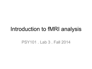
![the blood oxygen level dependent (BOLD) response
300 10 20
0
time [s]
peak
undershoot
hemodynamic
lag
stimulus](https://image.slidesharecdn.com/psy101lab3slides-150327172459-conversion-gate01/85/Introduction-to-fMRI-7-320.jpg)
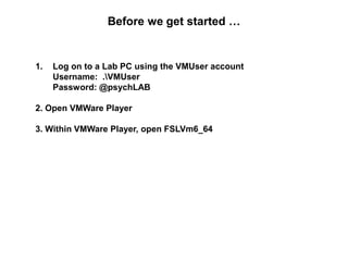
![time [s]
BOLD
stimulus
the BOLD response over time](https://image.slidesharecdn.com/psy101lab3slides-150327172459-conversion-gate01/85/Introduction-to-fMRI-8-320.jpg)
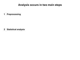
![A [BOLD] response is measured for every voxel](https://image.slidesharecdn.com/psy101lab3slides-150327172459-conversion-gate01/85/Introduction-to-fMRI-9-320.jpg)
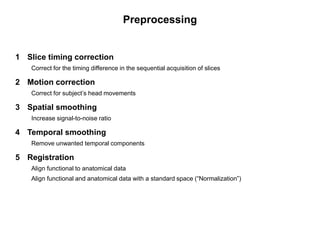
![Outline of a scan session
1 Task instruction + safety screening
2 Put subject in the scanner
3 Localizer scan
4 Anatomical scan
5 Shimming
6 Test scan
7 Data collection
8 [Field map]](https://image.slidesharecdn.com/psy101lab3slides-150327172459-conversion-gate01/85/Introduction-to-fMRI-11-320.jpg)
![Slice-timing correction
• In our experiment we measured one
functional image (volume) of the brain every 2
seconds
• Each volume was acquired in 36 interleaved
horizontal slices
• This means that every slice was acquired at a
different time during the 2s TR
Space[slices]
time [s]
volume (TR) volume (TR)
1
36
18](https://image.slidesharecdn.com/psy101lab3slides-150327172459-conversion-gate01/85/Introduction-to-fMRI-20-320.jpg)
![Slice-timing correction
To correct for this difference in timing, time-
series in each slice is phase-shifted so that it
appears as if all slices were acquired at the
same time
Space[slices]
time [s]
volume (TR) volume (TR)
1
36
18](https://image.slidesharecdn.com/psy101lab3slides-150327172459-conversion-gate01/85/Introduction-to-fMRI-21-320.jpg)
![roll [°] pitch [°] yaw [°] I-S [mm] R-L [mm] A-P [mm]
Rotation Translation
Motion correction output](https://image.slidesharecdn.com/psy101lab3slides-150327172459-conversion-gate01/85/Introduction-to-fMRI-24-320.jpg)
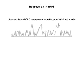
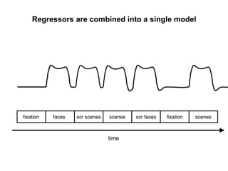
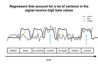
![Statistical analysis: regression
Core idea: observed data can be explained by a combination of weighted
regressors
Example: Explain miles per gallon (mpg) of a car, based on the car’s weight
and the driver’s height.
Observed data: mpg
Regressors: car’s weight, driver’s height
Weights: βcar’s weight = high; βdriver’s height = low
0
5
10
15
20
25
30
2 2.5 3 3.5 4 4.5 5
0
5
10
15
20
25
30
1.4 1.6 1.8 2 2.2
mpg
mpg
Driver’s height [m]Car’s weight [t]](https://image.slidesharecdn.com/psy101lab3slides-150327172459-conversion-gate01/85/Introduction-to-fMRI-28-320.jpg)

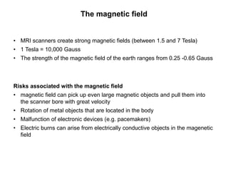
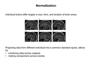
This document provides an overview of MRI/fMRI technology, including the operational principles of MRI scanners and their associated risks, such as the effects of powerful magnetic fields. It discusses the methodology of fMRI data collection and analysis, emphasizing preprocessing steps like motion correction and spatial normalization, as well as statistical analysis techniques. Additionally, it outlines the experimental setup for a fMRI lab session, focusing on task instructions and the analysis of neural responses to various visual stimuli.