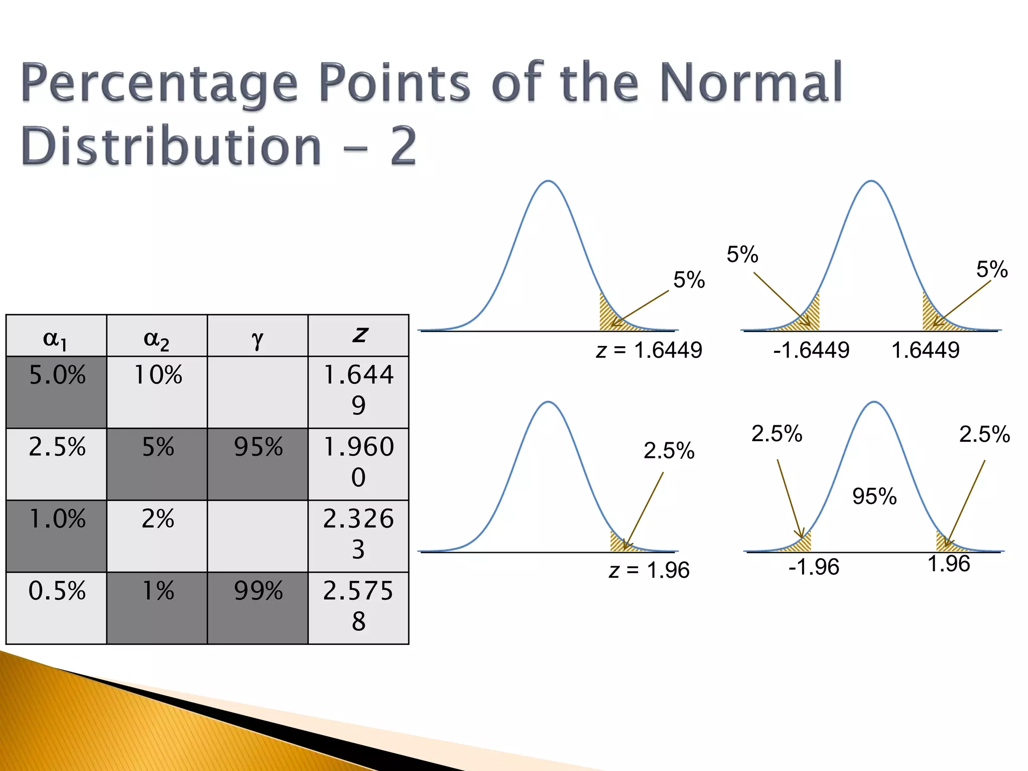
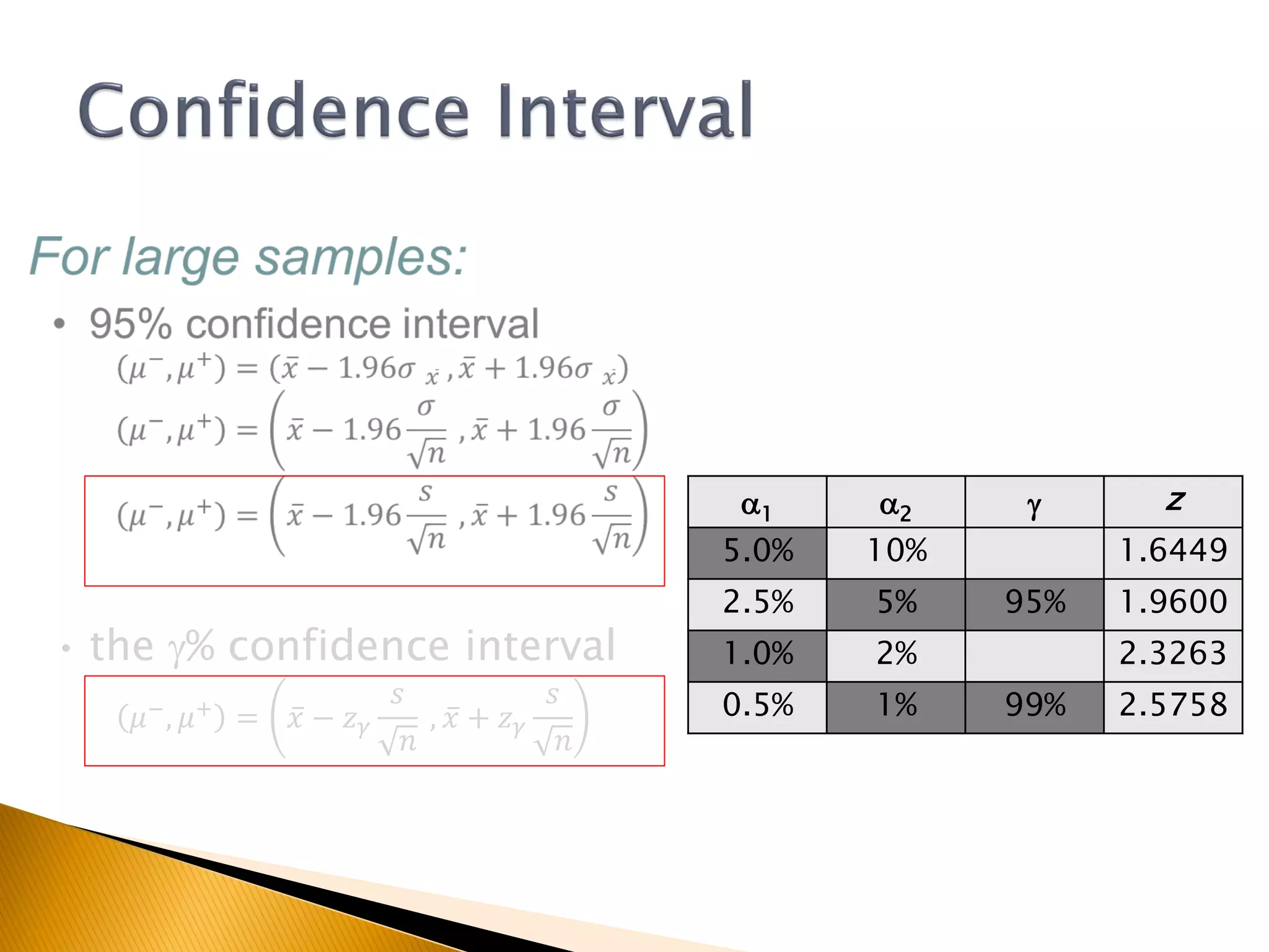
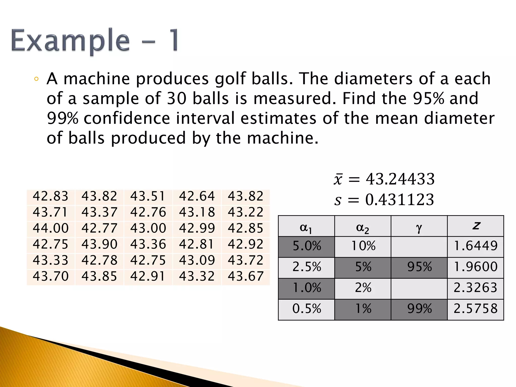
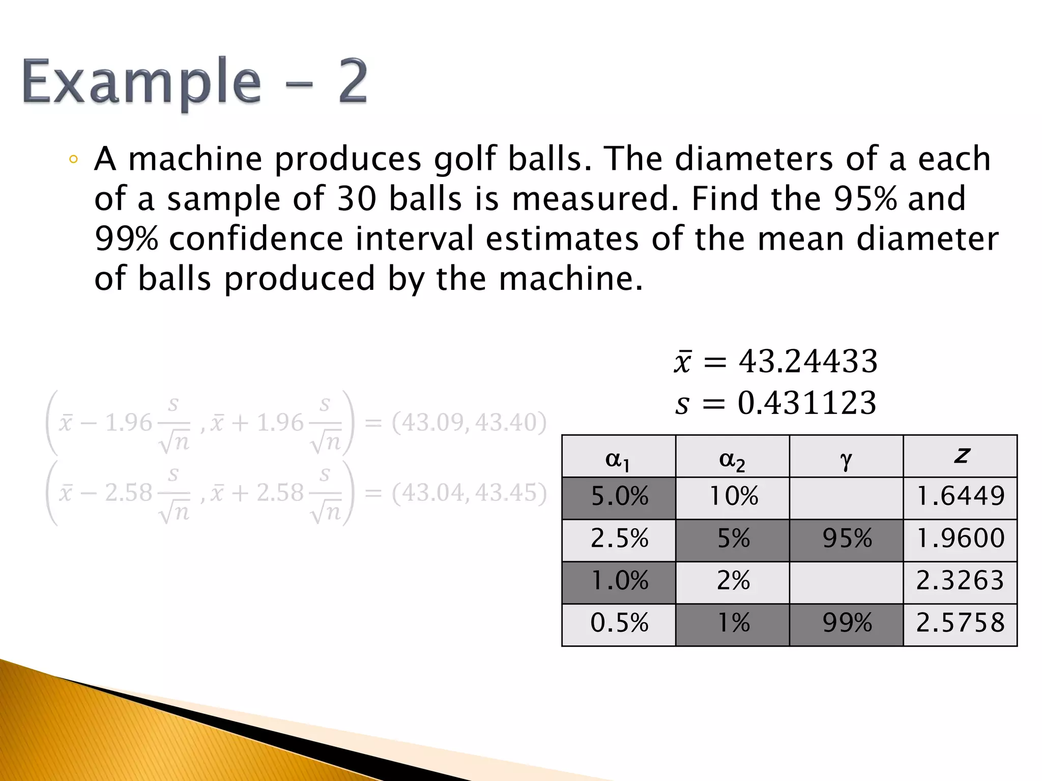
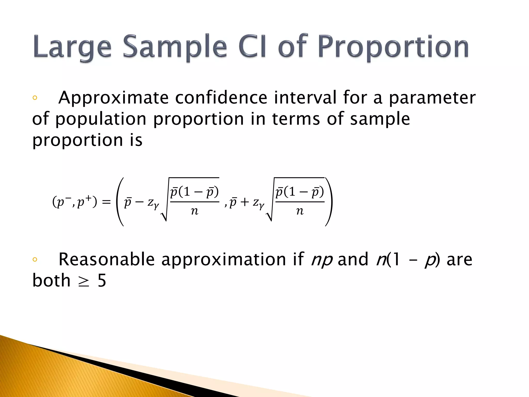
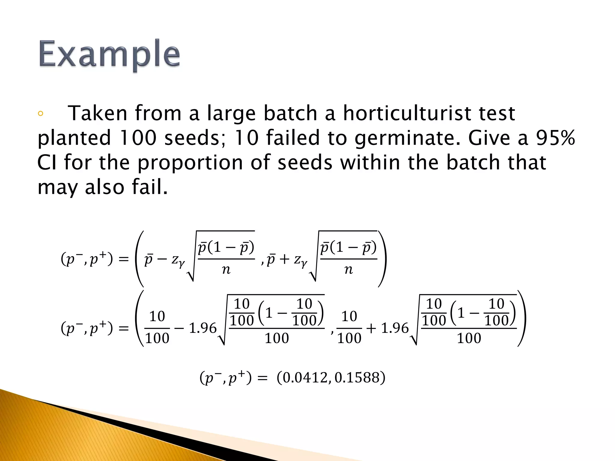
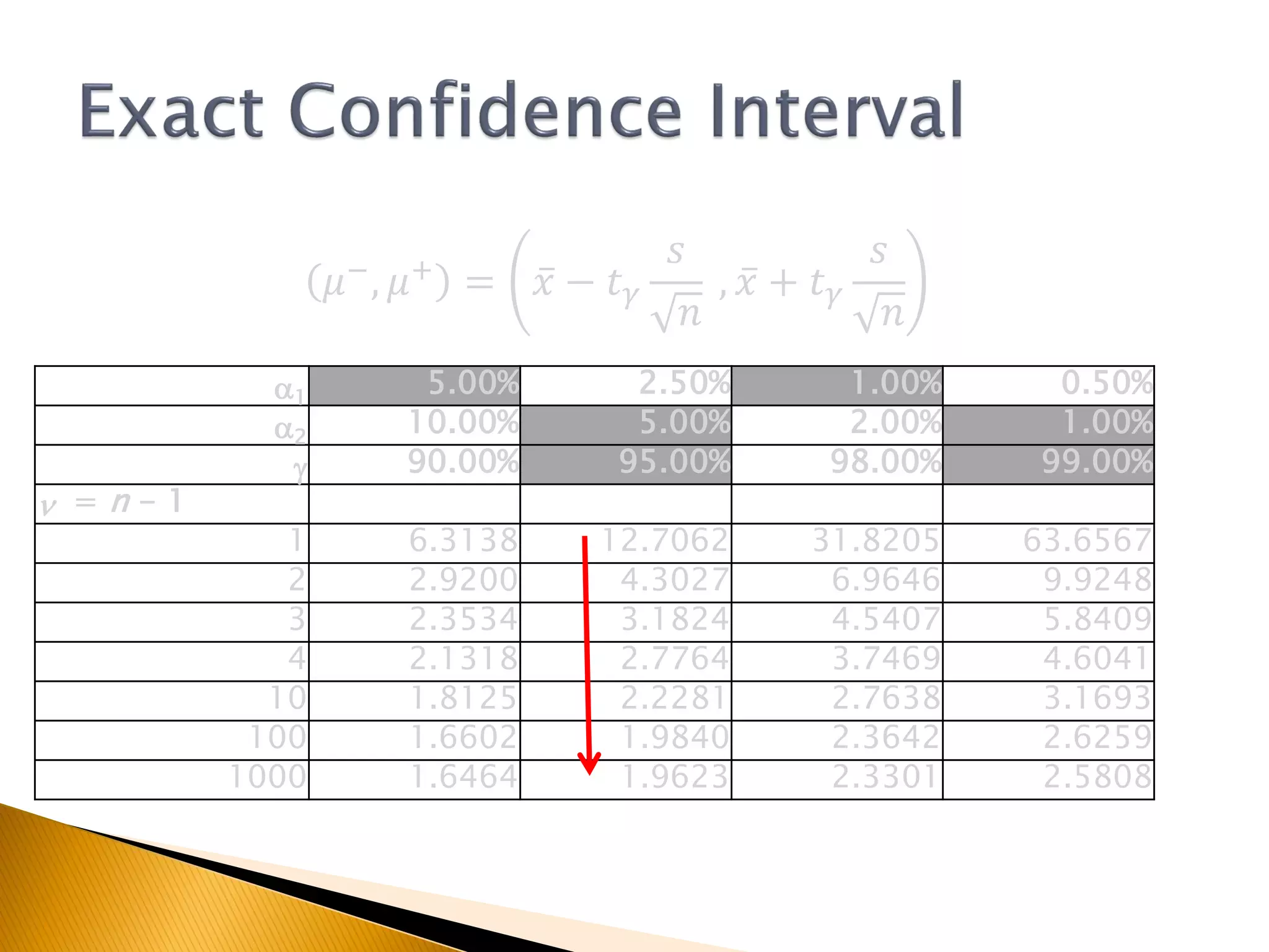
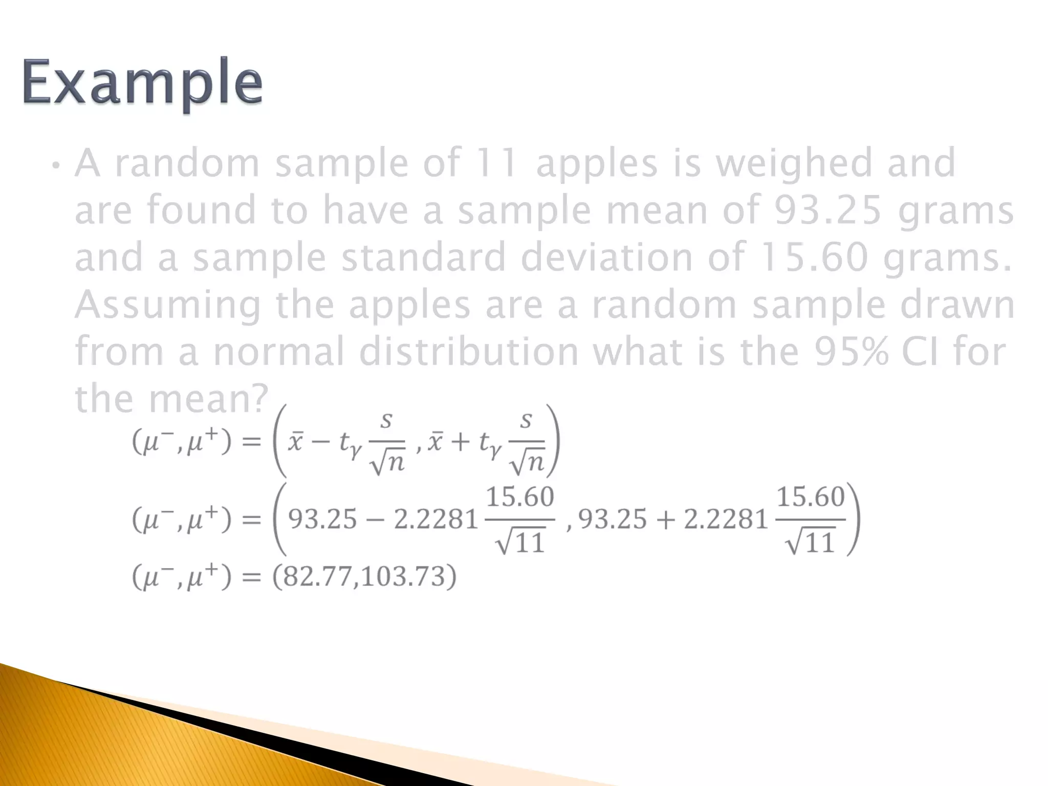
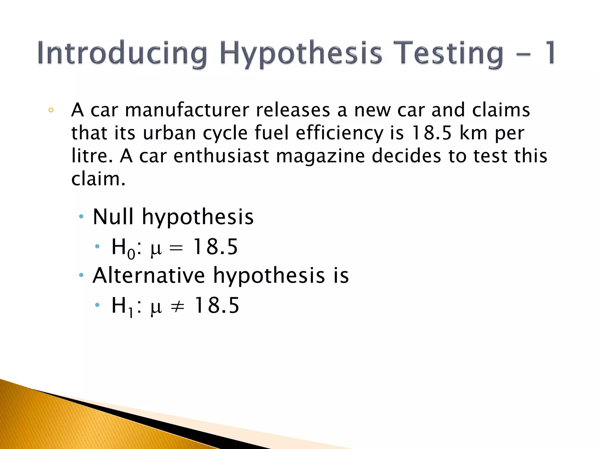
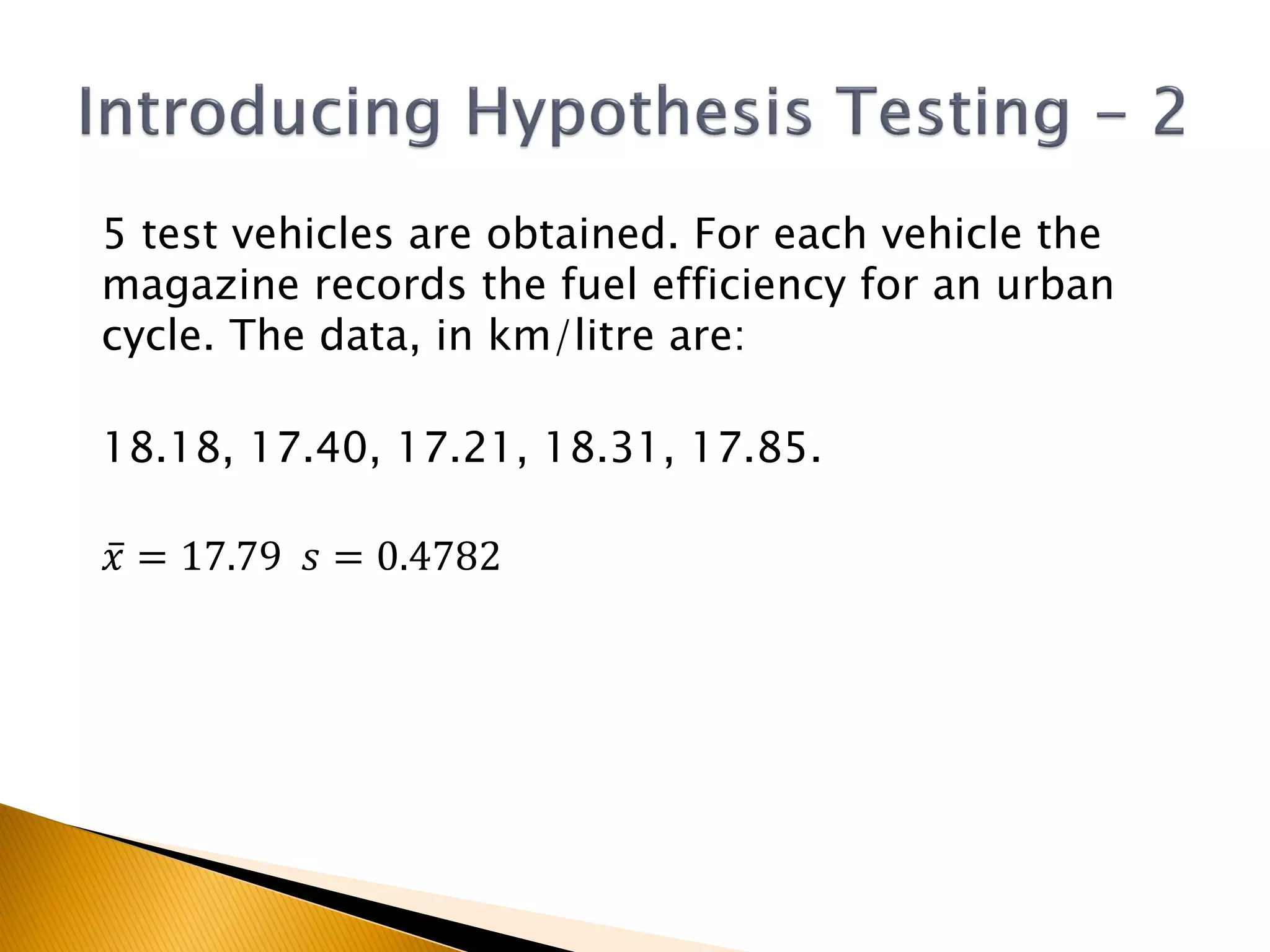
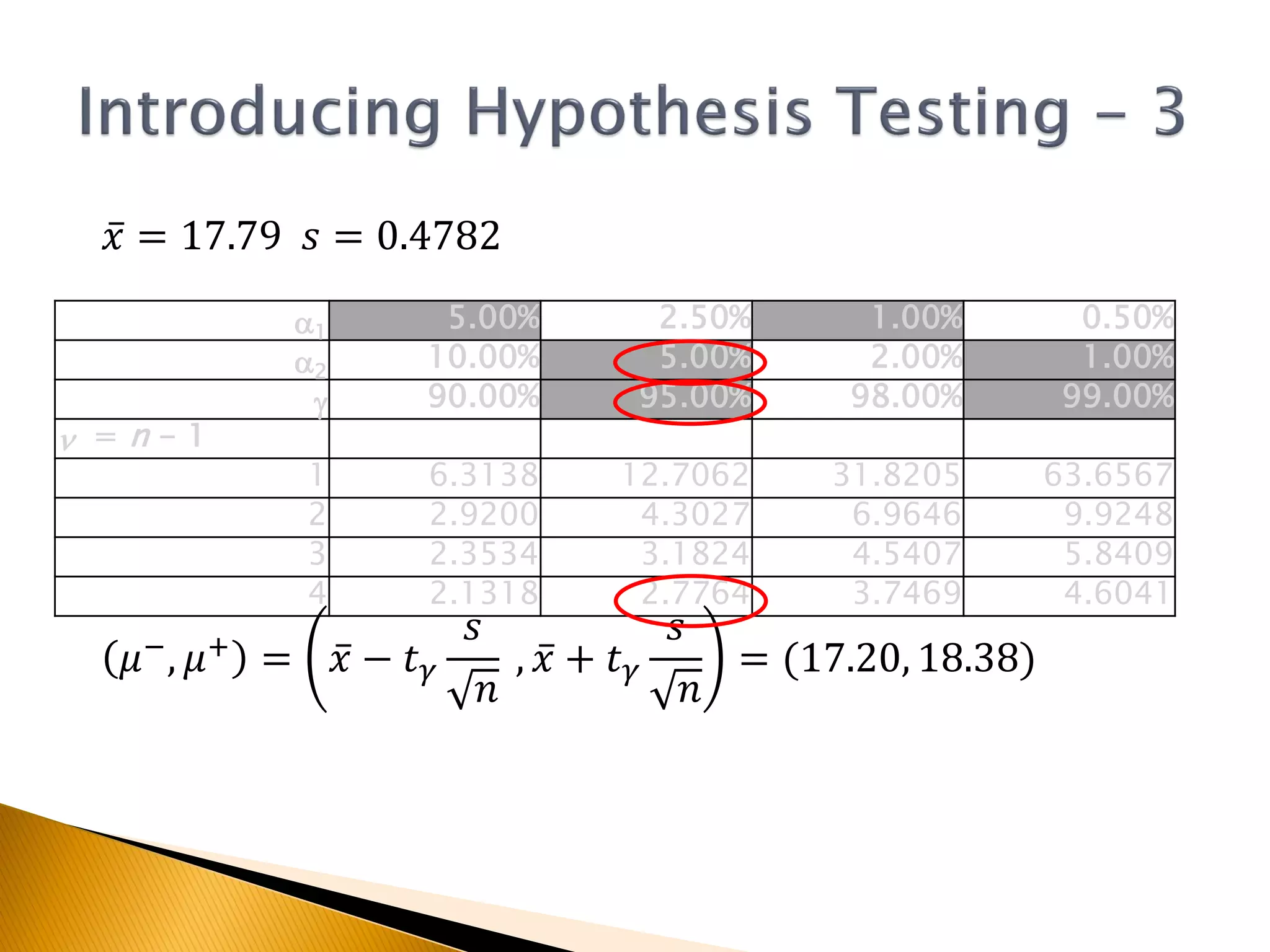
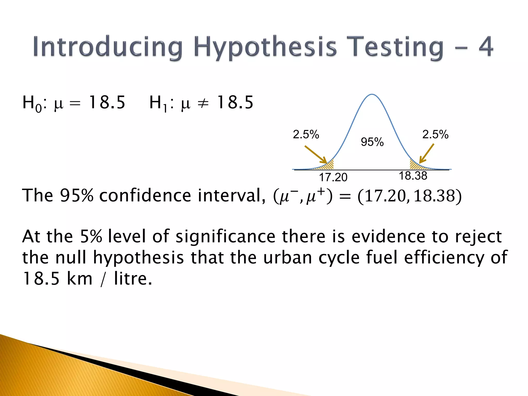
This document covers inferential statistics, including sampling distributions, point estimates, confidence intervals, and hypothesis testing. It provides formulas for calculating confidence intervals, examples involving golf ball measurements and apple weights, and discusses null and alternative hypotheses with real-world applications. By the end of the topic, students should be able to recognize key statistical terms and apply confidence intervals appropriately.

1. Topic 3:
Inferential Statistics 1

2. This topic will cover:
◦ Sampling distributions
◦ Point estimates and confidence intervals
◦ Introduction to hypothesis testing

3. By the end of this topic students will be able
to:
◦ Recognise the terms sample statistic and
population parameter
◦ Use confidence intervals to indicate the reliability of
estimates
◦ Know when approximate large sample or exact
confidence intervals are appropriate

4. P(Z < 1)
= 0.8413
P( - 1 <Z <
1) = 0.6826
z = 1.0
P(Z > 1)
= 0.1587
m
P( 0 <Z < 1)
= 0.3413
m + s x
𝑧 =
𝑥 − 𝜇
𝜎
0.0 1.0 -1.0 1.0

5. P(Z < 1)
= 0.8413
z = 1.0m m + s x
P( - 1 <Z <
1) = 0.6826
P( 0 <Z <
1) = 0.3413
0.0 1.0 -1.0 1.0
z 0 1 2 3
0.8 0.788
1
0.791
0
0.793
9
0.796
7
0.9 0.815
9
0.818
6
0.821
2
0.823
8
1.0 0.841
3
0.843
8
0.846
1
0.848
5
1.1 0.864
3
0.866
5
0.868
6
0.870
8
z 0 1 2 3
0.8 0.288
1
0.291
0
0.293
9
0.296
7
0.9 0.315
9
0.318
6
0.321
2
0.323
8
1.0 0.341
3
0.343
8
0.346
1
0.348
5
1.1 0.364
3
0.366
5
0.368
6
0.370
8

6. 5%
z = 1.6449
z = 1.96
5%
5%
2.5%
2.5%2.5%
P(Z > 1.6449) = 0.05
1.6449-1.6449
-1.96 1.96
95%

7. 5%
z = 1.6449
z = 1.96
5%
5%
2.5%
2.5%2.5%
1.6449-1.6449
-1.96 1.96
95%
a1 a2 g z
5.0% 10% 1.644
9
2.5% 5% 95% 1.960
0
1.0% 2% 2.326
3
0.5% 1% 99% 2.575
8

8. Population Parameters
Sample
Statistics?
?

9. ◦ Population Parameter
◦ mean
𝜇 =
𝑓𝑖 𝑥𝑖
𝑁
◦ standard deviation
𝜎 =
𝑓𝑖 𝑥𝑖 − 𝜇 2
𝑁
◦ Sample Statistic
◦ sample mean
𝑥 =
𝑓𝑖 𝑥𝑖
𝑛
◦ sample standard
deviation
𝑠 =
𝑓𝑖 𝑥𝑖 − 𝜇 2
𝑛 − 1

10. Population Distribution
Distribution of Sample Means
m
s
𝑥𝜇 𝑥
𝜎𝑥
𝜇 𝑥 = 𝜇
𝜎𝑥 =
𝜎
𝑛

11. n > 30
Population Distribution Distribution of Sample Means

12. Population Parameters
Sample
Statistics
?

13. 95%
z = -1.96 z = 1.96

14. 𝑥 = 𝜇 𝑥 − 1.96𝜎 𝑥 𝑥 = 𝜇 𝑥 + 1.96𝜎 𝑥
With probability 0.95 the
sample mean 𝑥 lies within
1.96 standard errors of
the population mean m
𝜇 = 𝜇 𝑥
95%
With probability 0.95 m
lies within 1.96 standard
errors of the sample
mean 𝑥

15. a1 a2 g z
5.0% 10% 1.6449
2.5% 5% 95% 1.9600
1.0% 2% 2.3263
0.5% 1% 99% 2.5758
• the g% confidence interval
𝜇−
, 𝜇+
= 𝑥 − 𝑧 𝛾
𝑠
𝑛
, 𝑥 + 𝑧 𝛾
𝑠
𝑛

16. 𝜇−, 𝜇+ = 𝑥 − 1.96
𝑠
𝑛
, 𝑥 + 1.96
𝑠
𝑛
1 in 20 chance of not
containing population
mean
19 in 20 chance of
containing population
mean
m

17. ◦ A machine produces golf balls. The diameters of a each
of a sample of 30 balls is measured. Find the 95% and
99% confidence interval estimates of the mean diameter
of balls produced by the machine.
42.83 43.82 43.51 42.64 43.82
43.71 43.37 42.76 43.18 43.22
44.00 42.77 43.00 42.99 42.85
42.75 43.90 43.36 42.81 42.92
43.33 42.78 42.75 43.09 43.72
43.70 43.85 42.91 43.32 43.67
𝑥 = 43.24433
𝑠 = 0.431123
a1 a2 g z
5.0% 10% 1.6449
2.5% 5% 95% 1.9600
1.0% 2% 2.3263
0.5% 1% 99% 2.5758

18. ◦ A machine produces golf balls. The diameters of a each
of a sample of 30 balls is measured. Find the 95% and
99% confidence interval estimates of the mean diameter
of balls produced by the machine.
𝑥 = 43.24433
𝑠 = 0.431123𝑥 − 1.96
𝑠
𝑛
, 𝑥 + 1.96
𝑠
𝑛
= 43.09, 43.40
𝑥 − 2.58
𝑠
𝑛
, 𝑥 + 2.58
𝑠
𝑛
= (43.04, 43.45)
a1 a2 g z
5.0% 10% 1.6449
2.5% 5% 95% 1.9600
1.0% 2% 2.3263
0.5% 1% 99% 2.5758

19. ◦ Approximate confidence interval for a parameter
of population proportion in terms of sample
proportion is
𝑝−
, 𝑝+
= 𝑝 − 𝑧 𝛾
𝑝 1 − 𝑝
𝑛
, 𝑝 + 𝑧 𝛾
𝑝 1 − 𝑝
𝑛
◦ Reasonable approximation if np and n(1 - p) are
both ≥ 5

20. ◦ Taken from a large batch a horticulturist test
planted 100 seeds; 10 failed to germinate. Give a 95%
CI for the proportion of seeds within the batch that
may also fail.
𝑝−
, 𝑝+
= 𝑝 − 𝑧 𝛾
𝑝 1 − 𝑝
𝑛
, 𝑝 + 𝑧 𝛾
𝑝 1 − 𝑝
𝑛
𝑝−
, 𝑝+
=
10
100
− 1.96
10
100
1 −
10
100
100
,
10
100
+ 1.96
10
100
1 −
10
100
100
𝑝−, 𝑝+ = 0.0412, 0.1588

21. •If normal model for population then
- exact sample confidence interval can be
calculated
- do not use z percentage points but t percentage
points
- t percentage points come from a family of
distributions called Student’s t-distribution
- family because t-distribution depends on
degrees of freedom n = (n – 1)

22. t(1)
t(30)
t(4)

23. 𝜇−, 𝜇+ = 𝑥 − 𝑡 𝛾
𝑠
𝑛
, 𝑥 + 𝑡 𝛾
𝑠
𝑛
a1
5.00% 2.50% 1.00% 0.50%
a2
10.00% 5.00% 2.00% 1.00%
g 90.00% 95.00% 98.00% 99.00%
n = n - 1
1 6.3138 12.7062 31.8205 63.6567
2 2.9200 4.3027 6.9646 9.9248
3 2.3534 3.1824 4.5407 5.8409
4 2.1318 2.7764 3.7469 4.6041
10 1.8125 2.2281 2.7638 3.1693
100 1.6602 1.9840 2.3642 2.6259
1000 1.6464 1.9623 2.3301 2.5808

24. •A random sample of 11 apples is weighed and
are found to have a sample mean of 93.25 grams
and a sample standard deviation of 15.60 grams.
Assuming the apples are a random sample drawn
from a normal distribution what is the 95% CI for
the mean?

25. ◦ A car manufacturer releases a new car and claims
that its urban cycle fuel efficiency is 18.5 km per
litre. A car enthusiast magazine decides to test this
claim.
 Null hypothesis
 H0: m = 18.5
 Alternative hypothesis is
 H1: m ≠ 18.5

26. 5 test vehicles are obtained. For each vehicle the
magazine records the fuel efficiency for an urban
cycle. The data, in km/litre are:
18.18, 17.40, 17.21, 18.31, 17.85.
𝑥 = 17.79 𝑠 = 0.4782

27. 𝑥 = 17.79 𝑠 = 0.4782
𝜇−, 𝜇+ = 𝑥 − 𝑡 𝛾
𝑠
𝑛
, 𝑥 + 𝑡 𝛾
𝑠
𝑛
= (17.20, 18.38)
a1
5.00% 2.50% 1.00% 0.50%
a2
10.00% 5.00% 2.00% 1.00%
g 90.00% 95.00% 98.00% 99.00%
n = n - 1
1 6.3138 12.7062 31.8205 63.6567
2 2.9200 4.3027 6.9646 9.9248
3 2.3534 3.1824 4.5407 5.8409
4 2.1318 2.7764 3.7469 4.6041

28. H0: m = 18.5 H1: m ≠ 18.5
The 95% confidence interval, 𝜇−
, 𝜇+
= (17.20, 18.38)
At the 5% level of significance there is evidence to reject
the null hypothesis that the urban cycle fuel efficiency of
18.5 km / litre.
2.5%2.5%
17.20 18.38
95%

29. By the end of this topic students will be able
to:
◦ Recognise the terms sample statistic and
population parameter
◦ Use confidence intervals to indicate the reliability of
estimates
◦ Know when approximate large sample and exact
confidence intervals are appropriate

30. • Dewhurst, F. Quantitative Methods for
Business and Management. McGraw-Hill.
• Hinton, PR. Statistics Explained Routledge
• Oakshot, L. Essential Quantitative Methods
for Business, Management and Finance.
Palgrave Macmillan.

31. Any Questions?