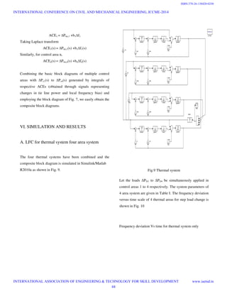
Iaetsd load frequency control for a distributed grid

LOAD FREQUENCY CONTROL FOR A DISTRIBUTED GRID
SYSTEM INVOLVING WIND, HYDRO AND THERMAL POWER
PLANTS
P Suresh Kumar Dr.K.Rama Sudha
PG scholar Professor
Department Electrical & Electronics Engineering,
Andhra University,
Visakhapatnam,
Andhra pradesh
Abstract- In an interconnected power system, as a
power load demand varies randomly both area
frequency and tie-line power interchange also vary. The
objectives of load frequency control (LFC) are to
minimize the deviations in these variables (area
frequency and tie-line power interchange) and to ensure
their steady state errors to be zero. In this area of
energy crisis, renewable energy is the most promising
solution to man’s ever increasing energy needs. But the
power production by these resources cannot be
controlled unlike in thermal plants. As a result,
standalone operation of renewable energy is not
reliable. Hence grid-connection of these along with
conventional plants is preferred due to the improved
performance in response to dynamic load. It is observed
that fluctuations in frequency caused due to load
variations are low with increase in penetration of
renewable resources. Load frequency control (LFC)
including PI controller is proposed in order to suppress
frequency deviations for a power system involving wind,
hydro and thermal plants owing to load and generating
power fluctuations caused by penetration of renewable
resources. A system involving four thermal plants, a
wind farm and a hydro plant will be modeled using
MATLAB.
Index Terms—Continuous power generation, load
frequency, Control (LFC), wind power, hydro power,
and thermal power plants LFC of multi area system,
Frequency deviation in the multi area system.
I. NOMENCLATURE
∆PC Command signal
∆F Frequency change
∆YE Changes in steam valve opening
R Speed regulation of the governor
Ksg Gain of speed governor
Tsg Time constant of speed governor
Rp Permanent droop
Rt Temporary droop
Tg Main servo time constant
D Change in load with respect to frequency
Tw Water starting time
Tr Reset time
Kt Gain of turbine
Tt Time constant of turbine
II. INTRODUCTION
The high Indian population coupled with increase in
industrial growth has resulted in an urgent need to increase
the installed power capacity. In India, majority of power
production, around 65 percent is from thermal power
stations. Due to problems related to uncertainty in pricing
and supply of fossil fuels, renewable resources have been
identified as a suitable alternative [7]. However, standalone
operation of renewable resources is not reliable as they are
intermittent in nature. The intermittent nature of resource
increases the frequency deviations which further add to the
deviation caused by load variation. This necessitates the
grid connection of renewable resources [4] [2]. Frequency
deviation is undesirable because most of the AC motors run
at speeds that are directly related to frequency. Also the
generator turbines are designed to operate at a very precise
speed. Microcontrollers are dependent on frequency for
their timely operation. Thus it is imperative to maintain
system frequency constant. This is done by implementing
Load Frequency Control (LFC). There are many LFC
methods developed for controlling frequency. They include
INTERNATIONAL CONFERENCE ON CIVIL AND MECHANICAL ENGINEERING, ICCME-2014
INTERNATIONAL ASSOCIATION OF ENGINEERING & TECHNOLOGY FOR SKILL DEVELOPMENT www.iaetsd.in
39
ISBN:378-26-138420-0245

flat frequency control (FFC), tie-line bias control (TBC)
and flat tie-line control (FTC) [1]. In FFC, Some areas act
as load change absorbers and others as base load. The
advantage is the higher operating efficiencies of the base
load as they run at their maximum rated value at all times.
But the drawback here is the reduced number of areas
absorbing load changes which makes the system more
transient prone. In FTC load changes in each area are
controlled within the area, thereby maintaining tie line
frequency constant. The most commonly used method is
the tie-line load bias control in which all power systems in
the interconnection aid in regulating frequency regardless
of where the frequency change originates. In this paper, the
power system considered has a Thermal system with four
thermal areas, a Hydro plant and a wind farm.
III. MODELING OF THERMAL AREAS
The thermal areas have been modeled using transfer
function. Speed governor, turbine and generator constitute
the various parts namely the speed governing system,
turbine model, generator load model .A complete block
diagram representation of an isolated power system
comprising Speed governor, turbine and generator and load
is easily obtained by combining the block diagrams of
individual components. [7].
A. Mathematical modeling of speed Governing
System
The command signal ∆PC initiates a sequence of events-the
pilot valve moves upwards, high pressure oil flows on to
the top of the main piston moving it downwards; the steam
valve opening consequently increases, the turbine generator
speed increases, i.e. the frequency goes up which is
modeled mathematically.
∆ܻாሺ‫ݏ‬ሻ = ቂ∆ܲ஼ሺ‫ݏ‬ሻ − ቀ
ଵ
ோ
ቁ ∗ ∆‫ܨ‬ሺ‫ݏ‬ሻቃ ∗ ሺ
௄ೞ೒
ଵା்ೞ೒∗௦
ሻ (1)
Fig 1.Block diagram representation of speed governing
system
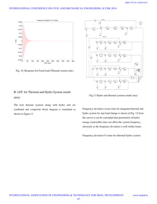
B. Mathematical modeling Turbine model
The dynamic response of steam turbine is related to
changes in steam valve opening ∆YE in terms of changes in
power output. Typically the time constant Tt lies in the
range 0.2 to 2.5 sec.
The dynamic response is largely influenced by two factors
(i) entrained steam between the inlet steam valve and first
Stage of the turbine,
(ii) The storage action in the reheater which causes the
Output of the low pressure stage to lag behind that of
the
High pressure stage
Fig 2.Turbine transfer function model
40
ISBN:378-26-138420-0246

C. Mathematical modeling Generator Load
Model
The increment in power input to the generator-load system
is related to frequency change as
∆‫ܨ‬ሺ‫ݏ‬ሻ = ሾ∆ܲீሺ‫ݏ‬ሻ − ∆ܲ஽ሺ‫ݏ‬ሻሿ ∗ ൬
௄೛ೞ
ଵା்೛ೞௌ
൰ (2)
Fig 3. Block diagram representation of generator-load
Model
D. Entire thermal area
Typical values of time constants of load frequency control
system are related as Tsg< Tt << Tps. Fig. 4 shows the
required block diagram and Table 1 shows the different
parameters of the four thermal areas.
Fig 4. Block diagram of entire thermal area
Table 1 Parameters of all four thermal areas
IV. MODELING OF HYDRO AND WIND
AREA
A. Modeling of hydro area
The representation of the hydraulic turbine and water
column in stability studies is usually based on certain
assumptions. The hydraulic resistance is considered
negligible. The penstock pipe is assumed inelastic and
water incompressible. Also the velocity of the water is
considered to vary directly with the gate opening and with
the square root of the net head and the turbine output power
is nearly proportional to the product of head and volume
flow [3]. Hydro plants are modeled the same way as
thermal plants. The input to the hydro turbine is water
instead of steam. Initial droop characteristics owing to
reduced pressure on turbine on opening the gate valve has
to be compensated. Hydro turbines have peculiar response
due to water inertia; a change in gate position produces an
initial turbine power change which is opposite to that
sought. For stable control performance, a large transient
(temporary) droop with a long resettling time is therefore
required in the forms of transient droop compensation as
shown in Fig. 5. The compensation limits gate movement
until water flow power output has time to catch up. The
41
ISBN:378-26-138420-0247

result is governor exhibits a high droop for fast speed
deviations and low droop in steady state.
Fig 5.Block diagram of hydro area.
B. Modeling of wind farm
Wind passes over the blades, generating lift and exerting a
turning force. The rotating blades turn a shaft inside the
nacelle, which goes into a gearbox. The gearbox increases
the rotational speed to that which is appropriate for the
generator, which uses magnetic fields to convert the
rotational energy into electrical energy. The power in the
wind that can be extracted by a wind turbine is proportional
to the cube of the wind speed and is given in watts by
P= ( Aν3
Cp)/2 where ρ is the air density, A is the rotor
swept area, ν is the wind speed and Cp is the power
coefficient. A maximum value of Cp is defined by the Betz
limit, which states that a turbine can never extract more
than 59.3% of the power from an air stream. In reality,
wind turbine rotors have maximum Cp values in the range
25–45%.
A wind farm consisting of Doubly-fed induction generator
(DFIG) wind turbine is considered. DFIG consists of a
wound rotor induction generator and an AC/DC/AC IGBT-
based PWM converter. The stator winding is connected
directly to the 50 Hz grid while the rotor is fed at variable
frequency through the AC/DC/AC converter. The wind
speed is maintained constant at 11 m/s. The control system
uses a torque controller in order to maintain the speed at 1.2
pu [6] [9] [10].
Fig 6. Block diagram of simple wind turbine
V. LFC FOR A MULTI-AREA SYSTEM
An extended power system can be divided into a number of
load frequency control areas interconnected by means of tie
lines. The control objective now is to regulate the frequency
of each area and to simultaneously regulate the tie line
power as per inter-area contacts. As in case of frequency,
proportional plus integral controller will be installed so as
to give zero steady state error in the tie line power flow as
compared to the contracted power. It is conveniently
assumed that each control area can be represented by an
equivalent turbine, generator and governor system.
Symbols used with suffix 1 refer to area 1 & those with
suffix 2 refer to area 2 and so on. Incremental tie line power
out of area 1 given by [5].
∆ܲ௧௜௘,ଵ = 2ߨܶଵଶሺ‫׬‬ ∆݂ଵ݀‫ݐ‬ − ‫׬‬ ∆݂ଶ݀‫ݐ‬ሻ (3)
Similarly, the incremental tie line power output of area 2
is given by
∆ܲ௧௜௘,ଶ = 2ߨܶଵଶሺ‫׬‬ ∆݂ଶ݀‫ݐ‬ − ‫׬‬ ∆݂ଵ݀‫ݐ‬ሻ (4)
Where T12 = synchronizing coefficient
f1 and f2 represent frequency of the respective area.
42
ISBN:378-26-138420-0248

∆ܲ௧௜௘,ଶሺܵሻ = −
ଶగ௔భమ்భమ
ௌ
∗ ሾ∆‫ܨ‬ଵሺ‫ݏ‬ሻ − ∆‫ܨ‬ଶሺ‫ݏ‬ሻሿ (5)
This has been represented by fig.7
Fig 7. Block diagram of Tie-line power flow
With the primary LFC loop a change in the system load
will result in a steady state frequency deviation, depending
on the governor speed regulation. In order to reduce the
frequency deviation to zero we must provide a reset action
by introducing an integral controller to act on the load
reference setting to change the speed set point. The integral
controller increases the system type by 1 which forces the
final frequency deviation to zero. The integral controller
gain must be adjusted for a satisfactory transient response.
It is seen from the above discussion that with the speed
governing system installed on each machine, the steady
load frequency characteristic for a given speed changer
setting has considerable droop, from no load to full load
.system frequency system specifications are rather stringent
and, therefore so much change in frequency cannot be
tolerated. In fact, it is expected that the steady change in
frequency will be zero. While steady state frequency can be
brought back to the scheduled value by adjusting speed
changer setting, the system could undergo intolerable
dynamic frequency changes with changes in load. It leads
to the natural suggestion that the speed changer setting be
adjusted automatically by monitoring the frequency
changes.
For purpose, a single from ∆f is fed through an integrator to
the speed changer resulting in block diagram configuration
shown .the system now modifies to a proportional plus
integral controller, which is well known from control
theory, gives zero steady state error.
Therefore In the case of an isolated control area, ACE (area
control error) is the change in area frequency which when
used in integral control loop forced the steady state
frequency error to zero. In order that the steady state tie line
power error in a two area control be made zero another
integral control loop (one for each area) must be introduced
to integrate the incremental tie line power signal and feed it
back to the speed changer as shown in Fig 8
Fig.8 Diagram for Proportional plus Integral Load
frequency Control
For free governor operation the steady change in system
frequency for a sudden change in load demand (Pd) is given
as
∆‫ܨ‬ሺ‫ݏ‬ሻ =
ି௄೛ೞ∆௉ವ/ೄ
൫ଵା்೛ೞ൯ା
಼ೞ೒಼೟಼೛ೞ
ೃ
൫భశ೅ೞ೒ೞ൯∗ሺభశ೅೟ೞሻ
(6)
This is accomplished by a single integrating block by
redefining ACE as a linear combination of incremental
frequency and tie line power. Thus for control area 1
43
ISBN:378-26-138420-0249

ACE1 = ∆Ptie,1 +b1∆f1
Taking Laplace transform
ACE1(s) = ∆Ptie,1(s) +b1∆f1(s)
Similarly, for control area n,
ACEn(s) = ∆Ptie,n(s) +bn∆fn(s)
Combining the basic block diagrams of multiple control
areas with ∆Pc1(s) to ∆Pcn(s) generated by integrals of
respective ACEs (obtained through signals representing
changes in tie line power and local frequency bias) and
employing the block diagram of Fig. 7, we easily obtain the
composite block diagrams.
VI. SIMULATION AND RESULTS
A. LFC for thermal system four area system
The four thermal systems have been combined and the
composite block diagram is simulated in Simulink/Matlab
R2010a as shown in Fig. 9. Fig.9 Thermal system
Let the loads ∆PD1 to ∆PD4 be simultaneously applied in
control areas 1 to 4 respectively. The system parameters of
4 area system are given in Table I. The frequency deviation
versus time scale of 4 thermal areas for step load change is
shown in Fig. 10
Frequency deviation Vs time for thermal system only
44
ISBN:378-26-138420-0250

Fig. 10. Response for Fixed load (Thermal system only)
B. LFC for Thermal and Hydro System (multi
area)
The four thermal systems along with hydro unit are
combined and composite block diagram is simulated as
shown in figure.11
Fig.11 Hydro and thermal systems (multi area)
Frequency deviation versus time for integrated thermal and
hydro system for step load change is shown in Fig. 12 from
the curves it can be concluded that penetration of hydro
energy (renewable) does not affect the system frequency
adversely as the frequency deviation is well within limits.
Frequency deviation Vs time for (thermal hydro) system
0 50 100 150 200 250 300 350 400 450 500
-0.025
-0.02
-0.015
-0.01
-0.005
0
0.005
0.01
0.015
0.02
0.025
Time (sec)
f(Hz)
Frequency Deviation Vs Time(s)
45
ISBN:378-26-138420-0251

Fig. 12. Response for Fixed load (thermal +hydro system)
C. LFC for Thermal, Hydro and Wind system
To compensate the intermittent nature of renewable, grid
connection of the same is imperative for reliable power
generation.
It is possible to divide an extended power system into sub
areas in which the generators are tightly coupled together so
as to form a coherent group, i.e. all the generators respond
in unison to changes in load or speed changer settings. Such
a coherent area is called control area in which frequency is
assumed to be same throughout in static and dynamic
conditions. For the purpose of developing a suitable control
strategy, a control area can be reduced to a single speed
governor, turbo generator and load system consisting of
four thermal areas, a hydro area and wind farm is controlled
by a controller. By a batch control, the load is divided
amongst various power plants in the ratio of their capacities
by control system. This entire power system is modeled as
shown in fig.13
Fig.13 LFC for Thermal, Hydro and Wind system
The four thermal areas and the hydro unit are combined
together in the ‘Thermal & Hydro’ subsystem which is
same as the model shown in Fig. 8. The output ∆F of this
subsystem gets reflected in the grid voltage. DFIG wind
farm draws supply for stator from grid and the changing
wind speeds has an impact on its output. Power from the
DFIG is fed to the grid via stator and rotor depending on
the wind speed. Higher the wind speed, higher is the power
output, rotor feeds power; lower the wind speed, power
output is low, hence rotor draws power from grid to have
constant power flow through stator.
Frequency Deviation (Hz) vs. Time(s) for the Integrated
System
46
ISBN:378-26-138420-0252

Fig. 14. Response for Fixed Load (Thermal + Hydro +
Wind Systems)
The output of wind farm is sent to the central control
system to calculate the load distribution over thermal
station. Random load of 1.7pu with maximum variation of
0.8pu is considered here. Frequency deviation versus Time
for Integrated Thermal, Hydro and Wind system for step
load change is shown in Fig. 14 Real time systems are best
described by introducing random load variation. From the
curves, it can be concluded that in an integrated system
with high penetration of renewable, frequency deviation has
increased. Nevertheless, it is within limits thereby making
renewable energy sources desirable.
VII. CONCLUSION
Load frequency control becomes more important, when a
large amount of renewable power supplies like wind power
generation are introduced. In this paper Load Frequency
Control with considerable penetration of renewable has
been analyzed in the presence of Thermal, Hydro and Wind
Systems with pi controller. It is observed that frequency
deviation is low when wind system is introduced into the
actual thermal systems, and it is within the tolerable limits
for fixed load variations. The loads are distributed among
different units using Tie Line Bias Control method of LFC
as it gives minimal frequency deviation.
VIII. REFERENCES
[1] R. Oba, G. Shirai, R. Yokoyama, T. Niimura, and G.
Fujita, “Suppression of Short Term Disturbances from
Renewable Resources by Load Frequency Control
Considering Different Characteristics of Power Plants”,
IEEE Power & Energy Society General Meeting, pp.1 –
7, Jul.2009.
[2] N. R. Ullah, T. Thiringer, and Daniel
Karlsson,“Temporary Primary Frequency Control
Support by Variable Speed Wind Turbines— Potential
And Applications”, IEEE Transactions on Power
Systems, vol.23, No.2, May 2008.
[3] P. Kundur, Power System Stability and Control, 1st
ed., New York: McGraw-Hill, 1993.
[4] L. Freris and D. Infield, Renewable Energy in Power
Systems, 1st ed., J.Wiley Sons Ltd., 2008.
[5] H. Saadat, Power System Analysis, 1st ed., Tata
McGraw- Hill, 2002.
[6] O. Anaya-Lara, N. Jenkins, J. Ekanayake, P.
Cartwright, M. Hughes, Wind Energy generation
Modeling and Control, 1st
ed., J. Wiley Sons Ltd.,
2009.
[7] O. Elgerd, Electric Energy Systems Theory An
Introduction, 2nd ed., Tata McGraw-Hill, 1983
[8] L.R. Chang-Chien, W.T. Lin and Y.C. Yin,
“Enhancing frequency response control by DFIGs in
The high wind penetrated power systems,” IEEE
Transactions on power systems, 2010
[9] G. Lalor, A. Mullane, and M. O’Malley, “Frequency
Control and wind turbine technologies,” IEEE Trans.
Power Syst., vol. 20, no. 4, pp. 1905–1913, Nov.
47
ISBN:378-26-138420-0253

2005.
[10] J. de Almeida and R. G. Lopes, “Participation of
Doubly fed induction wind generators in system
Frequency regulation,” IEEE Trans. Power Syst., vol.
22, no. 3, pp. 944–950, Aug. 2007.
48
ISBN:378-26-138420-0254

Iaetsd load frequency control for a distributed grid

More Related Content

What's hot

Viewers also liked

Similar to Iaetsd load frequency control for a distributed grid

More from Iaetsd Iaetsd

Recently uploaded

Iaetsd load frequency control for a distributed grid