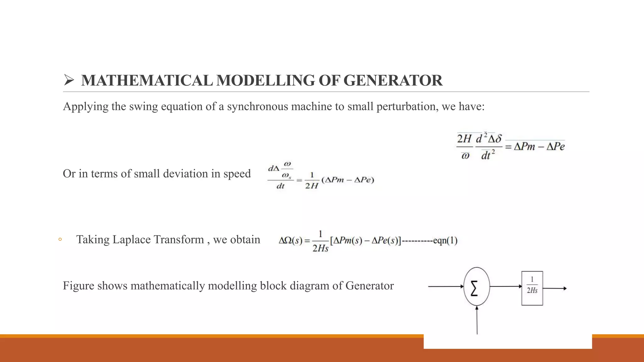
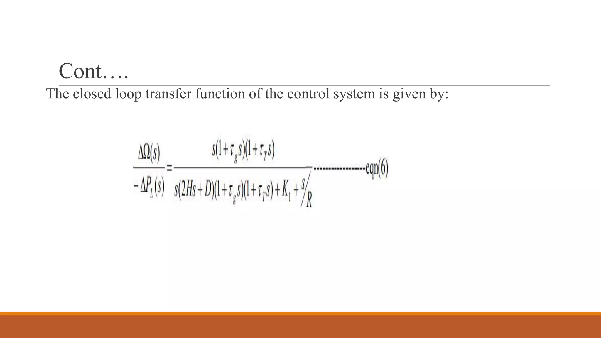
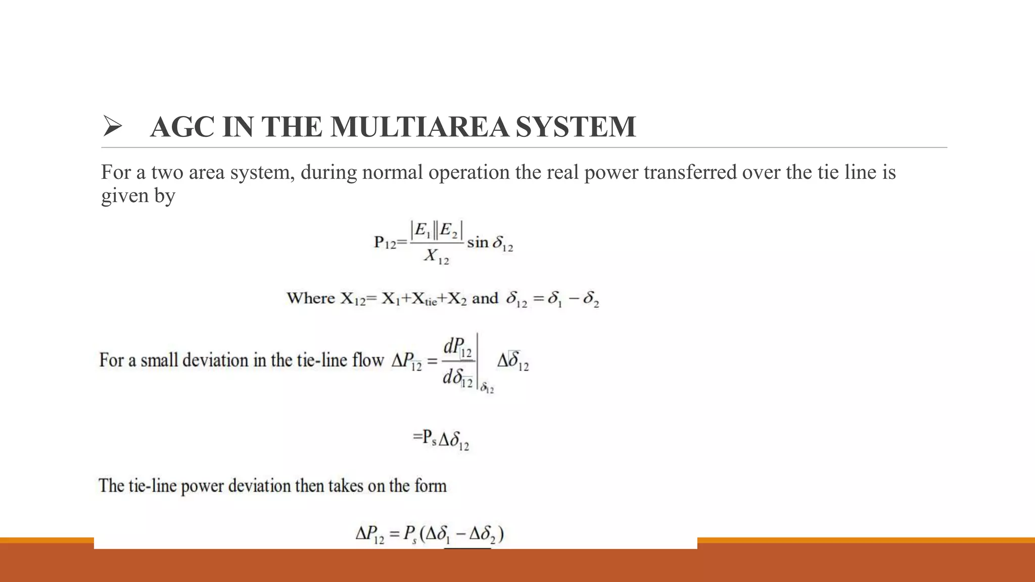
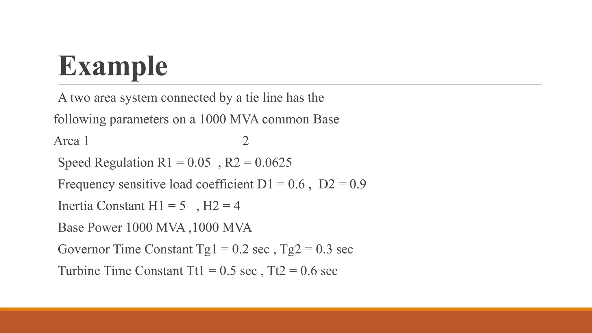
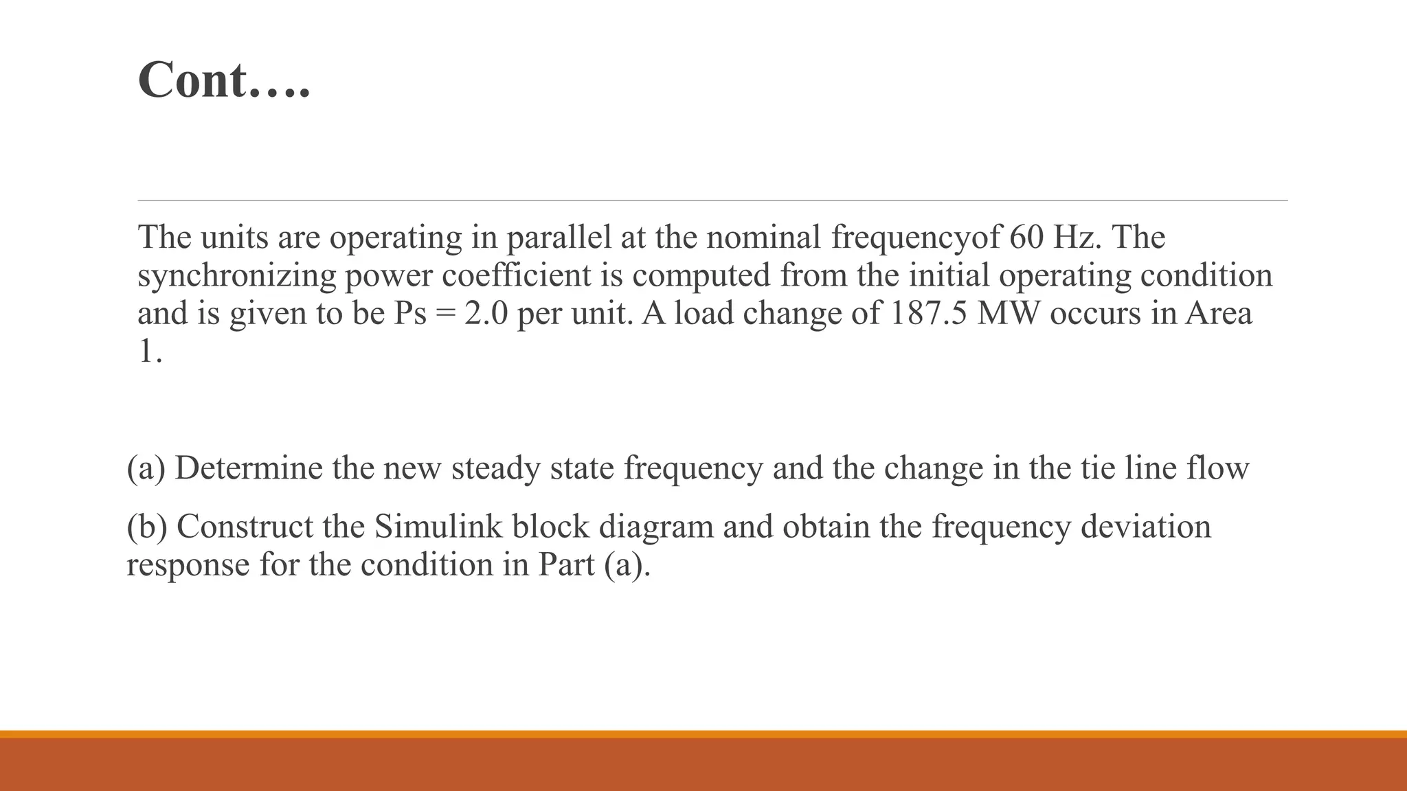
1) The document presents a case study on using electric vehicles to provide load frequency control in an interconnected power system. It discusses mathematical modeling of system components like generators, loads, prime movers, and governors. 2) The example given is of a two area power system where a 187.5 MW load change occurs in Area 1. The steady state frequency deviation and tie line power change are calculated. 3) Simulation results show a frequency deviation of -0.3 Hz and no change in tie line power for the given load change condition in Area 1. However, practically only the generator in Area 1 should respond, not both generators.

1. Presentation
LOAD FREQUENCY CONTROL USING ELECTRIC VEICHLE
SYSTEM IN INTERCONNECTED POWER SYSTEM
Gautam Buddha University Noida
Presented by :-
Narendra
M-Tech (Power System)
Department Of Electrical Engineering

2. Table of Contents
1.Introduction
2.Background &Literature Review
3.System Model
4.Example(Problem Statement)
5.Result &Analysis
6.Conclusions
7.Refrences

3. Introduction
For large scale power systems which consists of inter-connected control areas, load
frequency then it is important to keep the frequency and inter area tie power near to
the scheduled values.
A well designed power system should be able to provide the acceptable levels of
power quality by keeping the frequency and voltage magnitude within tolerable
limits. Changes in the power system load affects mainly the system frequency,
while the reactive power is less sensitive to changes in frequency and is mainly
dependent on fluctuations of voltage magnitude. So the control of the real and
reactive power in the power system is dealt separately.
The load frequency control mainly deals with the control of the system frequency
and real power whereas the automatic Voltage regulator loop regulates the changes
in the reactive power and voltage magnitude. Load frequency control is the basis of
many advanced concepts of the large scale control of the power system

4. BACKGROUND AND LITERARTURE REVIEW
Reasons for the Limits on Frequency:
Following are the reasons for keeping a strict limit on the system frequency variation:
The speed of the alternating current motors depends on the frequency of the power supply. There
are situations where speed consistency is expected to be of high order.
The electric clocks are driven by the synchronous motors. The accuracy of the clocks are not
only dependent on the frequency but also is an integral of the this frequency error.
The most serious effect of subnormal frequency operation is observed in the case of Thermal
Power Plants. Due to the subnormal frequency operation the blast of the ID and FD fans in the
power stations get reduced and thereby reduce the generation power in the thermal plants.

5.  LOAD FREQUENCY CONTROLAND MATHEMATICAL
MODELLING OFVARIOUS COMPONENTS:
If the system is connected to a number of different loads in a power system then the system
frequency and speed change with the governor characteristics as the load changes. If it is not
required to keep the frequency constant in a system then the operator is not required to change the
setting of the generator. The possibility of sharing the load by two machines is as follow:
Suppose there are two generating stations that are connected to each other by tie line. If the
change in load is either at A or at B and the generation of A is alone asked to regulate so as to
have constant frequency then this kind of regulation is called Flat Frequency Regulation.
The other possibility of sharing the load the load is that both A and B would regulate their
generations to maintain the constant frequency. This is called parallel frequency regulation.
The third possibility is that the change in the frequency of a particular area is taken care of by
the generator of that area thereby the tie-line loading remains the same. This method is known as
flat tie-line loading control.
The first step to the analysis of the control system is the mathematical modeling of the system’s
various components and control system techniques.

6.  MATHEMATICAL MODELLING OF GENERATOR
Applying the swing equation of a synchronous machine to small perturbation, we have:
Or in terms of small deviation in speed
◦ Taking Laplace Transform , we obtain
Figure shows mathematically modelling block diagram of Generator

7.  MATHEMATICAL MODELLING OF LOAD
The speed-load characteristic of the composite load is given by
Mathematically block diagram of Load
e

8.  MATHEMATICAL MODELLING FOR PRIME MOVER:
The source of power generation is commonly known as the prime mover. It may be hydraulic
turbines at waterfalls, steam turbines whose energy comes from burning of the coal, gas and other
fuels. The model for the turbine relates the changes in mechanical power output ΔPm to the
changes in the steam valve position ΔPV.

9.  MATHEMATICAL MODELLING FOR GOVERNOR
When the electrical load is suddenly increased then the electrical power exceeds the mechanical power input. As
a result of this the deficiency of power in the load side is extracted from the rotating energy of the turbine. Due to
this reason the kinetic energy of the turbine i.e. the energy stored in the machine is reduced and the governor
sends a signal to supply more volumes of water or steam or gas to increase the speed of the prime-mover so as to
compensate speed deficiency.
The slope of the curve represents speed regulation R. Governors typically have a speed regulation of 5-6 % from
no load to full load.

10. Cont…..
Or in s- domain

11. Cont…..
Combining all the block diagrams from earlier block diagrams for a single are system we get the
following:

12. System Model
AGC IN A SINGLE AREA:
With the primary LFC loop a change in the system load will result in a steady state frequency deviation
, depending on the governor speed regulation. In order to reduce the frequency deviation to zero we
must provide a reset action by introducing an integral controller to act on the load reference setting to
change the speed set point. The integral controller increases the system type by 1 which force the final
frequency deviation to zero. The integral controller gain must be adjusted for a satisfactory transient
response.

13. Cont….
The closed loop transfer function of the control system is given by:

14.  AGC IN THE MULTIAREA SYSTEM
For a two area system, during normal operation the real power transferred over the tie line is
given by

15. Cont….

16. Example
A two area system connected by a tie line has the
following parameters on a 1000 MVA common Base
Area 1 2
Speed Regulation R1 = 0.05 , R2 = 0.0625
Frequency sensitive load coefficient D1 = 0.6 , D2 = 0.9
Inertia Constant H1 = 5 , H2 = 4
Base Power 1000 MVA ,1000 MVA
Governor Time Constant Tg1 = 0.2 sec , Tg2 = 0.3 sec
Turbine Time Constant Tt1 = 0.5 sec , Tt2 = 0.6 sec

17. Cont….
The units are operating in parallel at the nominal frequencyof 60 Hz. The
synchronizing power coefficient is computed from the initial operating condition
and is given to be Ps = 2.0 per unit. A load change of 187.5 MW occurs in Area
1.
(a) Determine the new steady state frequency and the change in the tie line flow
(b) Construct the Simulink block diagram and obtain the frequency deviation
response for the condition in Part (a).

18. Result &Analysis
Steady State Frequency Deviation & Change in Tie Line Power.
The speed regulation of Area 1 and 2 is given by:
1/R1= 1/0.05= 20
1/R2= 1/0.0625=16
The inertia and load for area 1 and 2 is given by:
1/2H1s+D1= 1/2*5s+0.6= 1/10s+0.6
1/2H2s+D2= 1/2*4s+0.9= 1/8s+0.9
The per unit load change in Area 1 is given by:
PL1=187.5/1000= 0.1875p.u
The per unit steady state frequency deviation is
w= - PL1/(D1+1/R1)+(D2+1/R2
= -0.1875/(20+0.6)+(16+0.9) = -0.005 p.u

19. Cont…..
Thus, the steady state frequency deviation in Hz is
f(actual)= f pu*f(base)
= -0.005*60 = -0.3Hz
F(actual)= f (original)+ f(actual)
=60-0.3 = 59.7 Hz
Hence, The file is opened and is run in the SIMULINK window.

20. Conclusion
The project presents a case study of designing a controller that can bear desirable results in a two area
power system when the input parameters to the system is changed.
Two methods of Load Frequency Control was studied taking an isolated power system into
consideration.
It may be noted that load of 187.5 MW is changed in Area 1 power system. However, from the results,
it has been observed that both generators have enhanced their generation to meet the increased load
demand.
Practically this is not true. In the real practice, if sudden load is changed in any area, then each area
has to absorb its own changes or in other words, it has to be supplied by the generator of that area
only.
It means that for a load change of 187.5 MW, the change in mechanical power of area 1 should be
increased to 187.5 MW only. Whereas, the change in mechanical power of area 2 must remain zero.
Furthermore, change in tie line power should also remain zero.
To do this, we need to do some changes in the model in such a way that change of load in any area
may cause the change of generation in that area only.

21. Refrences
I.J. Nagrath and M.Gopal “ Control System Engineering” Fifth Edition, New Age International
Publisher, New Delhi.
C.L.Wadhwa, “Electrical Power system”, Sixth Edition, , New Age International Publisher, New
Delhi.
Hadi Saadat :”Power system analysis” Tata McGraw Hill 2002 Edition, New Delhi.
Malik,O.P., Kumar,A., and Hope,G.S., “A load frequency control algorithm based on generalized
approach”, IEEE Trans. On Power Systems, Vol 3,No.2, pp. 375-382,1998.