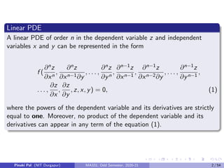
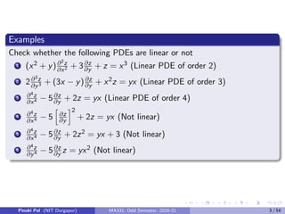
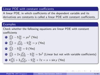
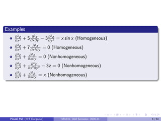
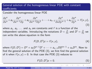
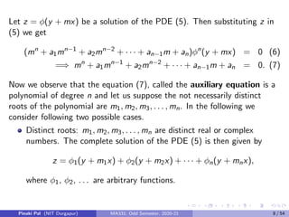
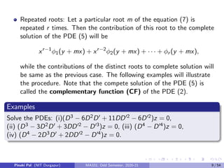
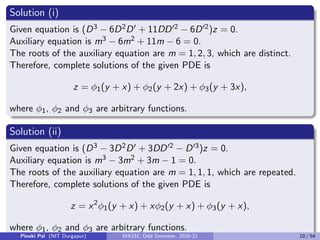
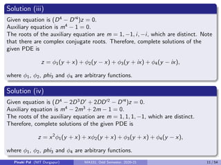
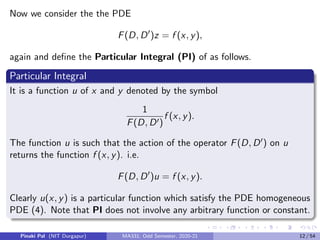
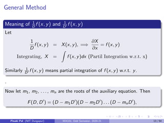
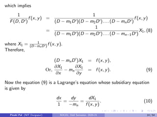
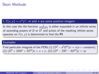
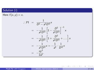
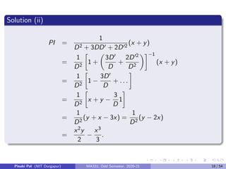
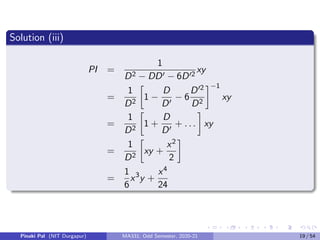
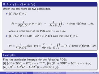
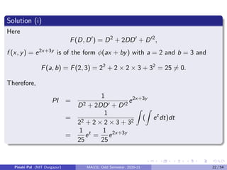
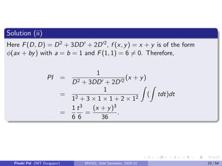
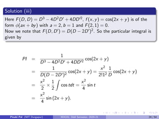
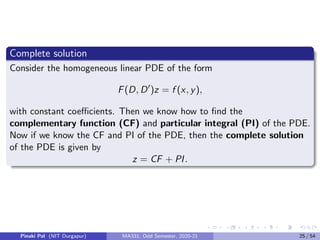
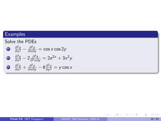
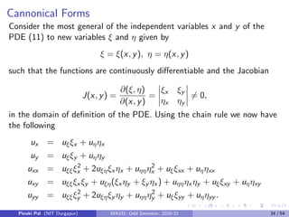
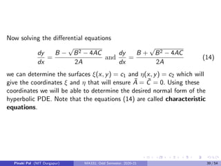
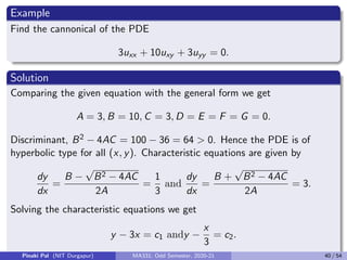
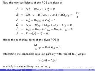
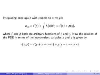
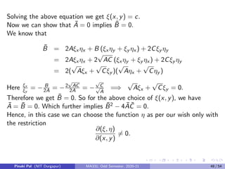
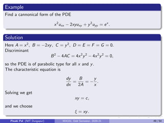
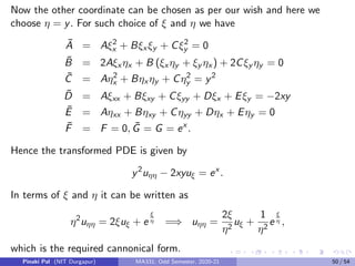
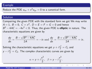
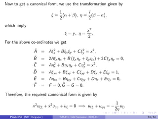
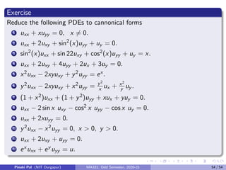
The document discusses linear partial differential equations (PDEs) with constant coefficients. It defines such PDEs and provides examples. It describes how to find the general solution of homogeneous linear PDEs with constant coefficients by finding the roots of the auxiliary equation. The general solution consists of the complementary function plus a particular integral. Methods for finding the particular integral when the right side consists of powers of x and y are also presented.


![Solution (i)
Auxiliary Equation is
m2
− m = 0 and the roots of it are m = 0, 1.
Therefore complementary function is z = φ1(y) + φ2(y + x).
Now
PI =
1
D2 − DD0
cos x cos 2y =
1
2
1
D2 − DD0
[cos(x + 2y) + cos(x − 2y)]
=
1
2
1
1 − 2
ZZ
cos tdtdt +
1
1 + 2
ZZ
cos t1dt1dt1
=
1
2
cos t −
1
3
cos t1
=
1
2
cos(x + 2y) −
1
6
cos(x − 2y)
Hence the complete solution is give by,
z = φ1(y) + φ2(y + x) +
1
2
cos(x + 2y) −
1
6
cos(x − 2y).
Pinaki Pal (NIT Durgapur) MA331; Odd Semester, 2020-21 27 / 54](https://image.slidesharecdn.com/lectures4-8-211221131700/85/Lectures4-8-27-320.jpg)
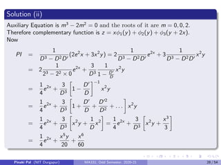
![So the complete solution is given by
z = xφ1(y) + φ2(y) + φ3(y + 2x +
1
4
e2x
+
x5y
20
+
x6
60
.
Solution (iii)
Auxiliary Equation is m2 + m − 6 = 0 and the roots of it are m = 2, −3.
Therefore complementary function is z = φ1(y + 2x) + φ2(y − 3x).
Now
PI =
1
D2 + DD0 − 6D02
y cos x =
1
(D + 3D0)(D − 2D0)
y cos x
=
1
(D + 3D0)
Z
(c − 2x) cos xdx [∵ y = c − 2x]
=
1
(D + 3D0)
[c sin x − 2x sin x − cos x]
=
1
(D + 3D0)
[(y + 2x) sin x − 2x sin x − cos x]
Pinaki Pal (NIT Durgapur) MA331; Odd Semester, 2020-21 29 / 54](https://image.slidesharecdn.com/lectures4-8-211221131700/85/Lectures4-8-29-320.jpg)
![∴ PI =
1
(D + 3D0)
[y sin x − cos x]
=
Z
[(c + 3x) sin x − cos x] dx [∵ y = c + 3x]
= −c cos x − sin x − 3x cos x + 3 sin x
= −(y − 3x) cos x − sin x − 3x cos x + 3 sin x
= −y cos x + 2 sin x
Hence the complete solution is given by
z = φ1(y + 2x) + φ2(y − 3x) − y cos x + 2 sin x.
Pinaki Pal (NIT Durgapur) MA331; Odd Semester, 2020-21 30 / 54](https://image.slidesharecdn.com/lectures4-8-211221131700/85/Lectures4-8-30-320.jpg)


![Week 4 [compatibility mode]](https://cdn.slidesharecdn.com/ss_thumbnails/week4compatibilitymode-130213165150-phpapp02-thumbnail.jpg?width=640&height=640&fit=bounds)


