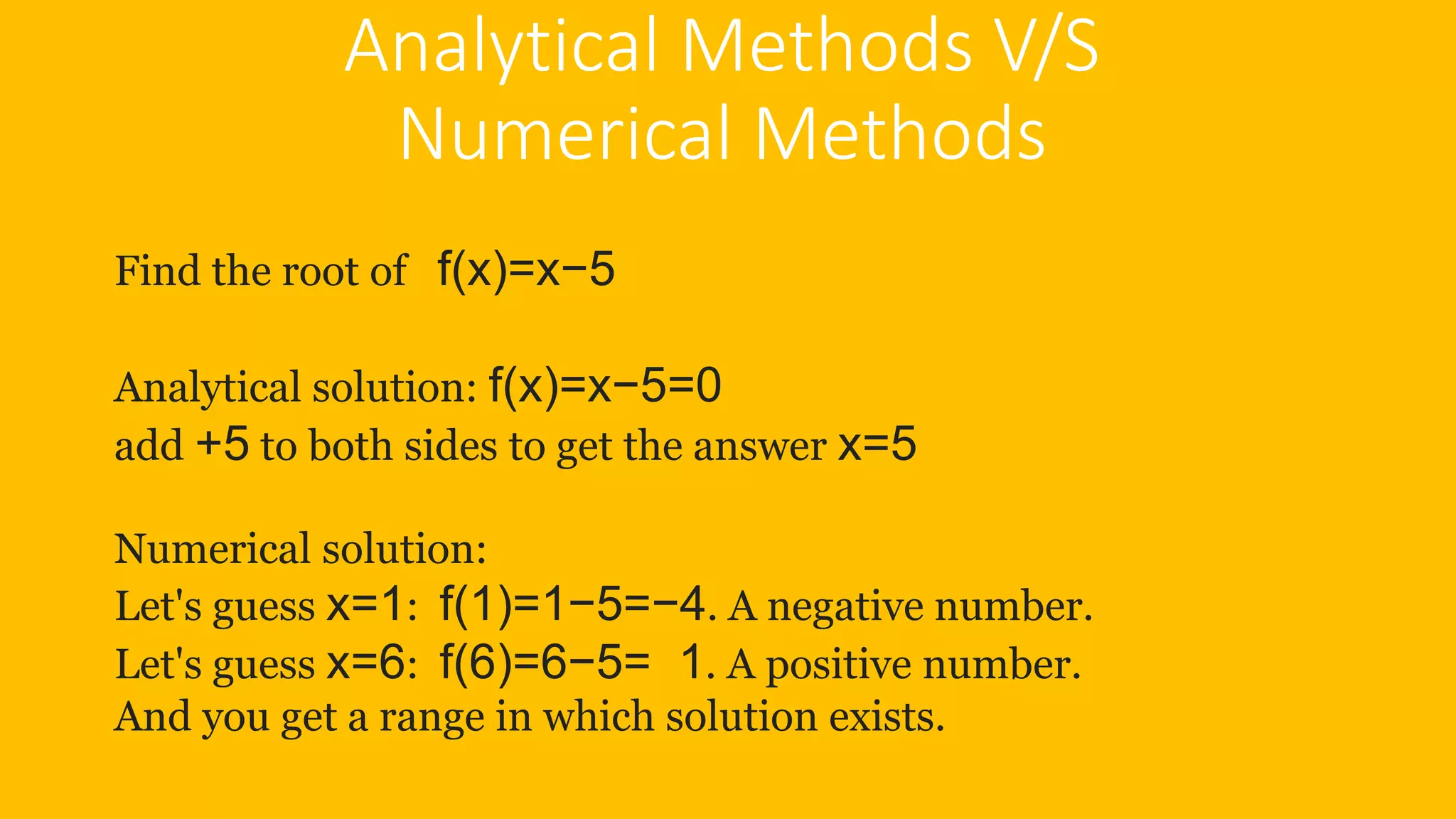
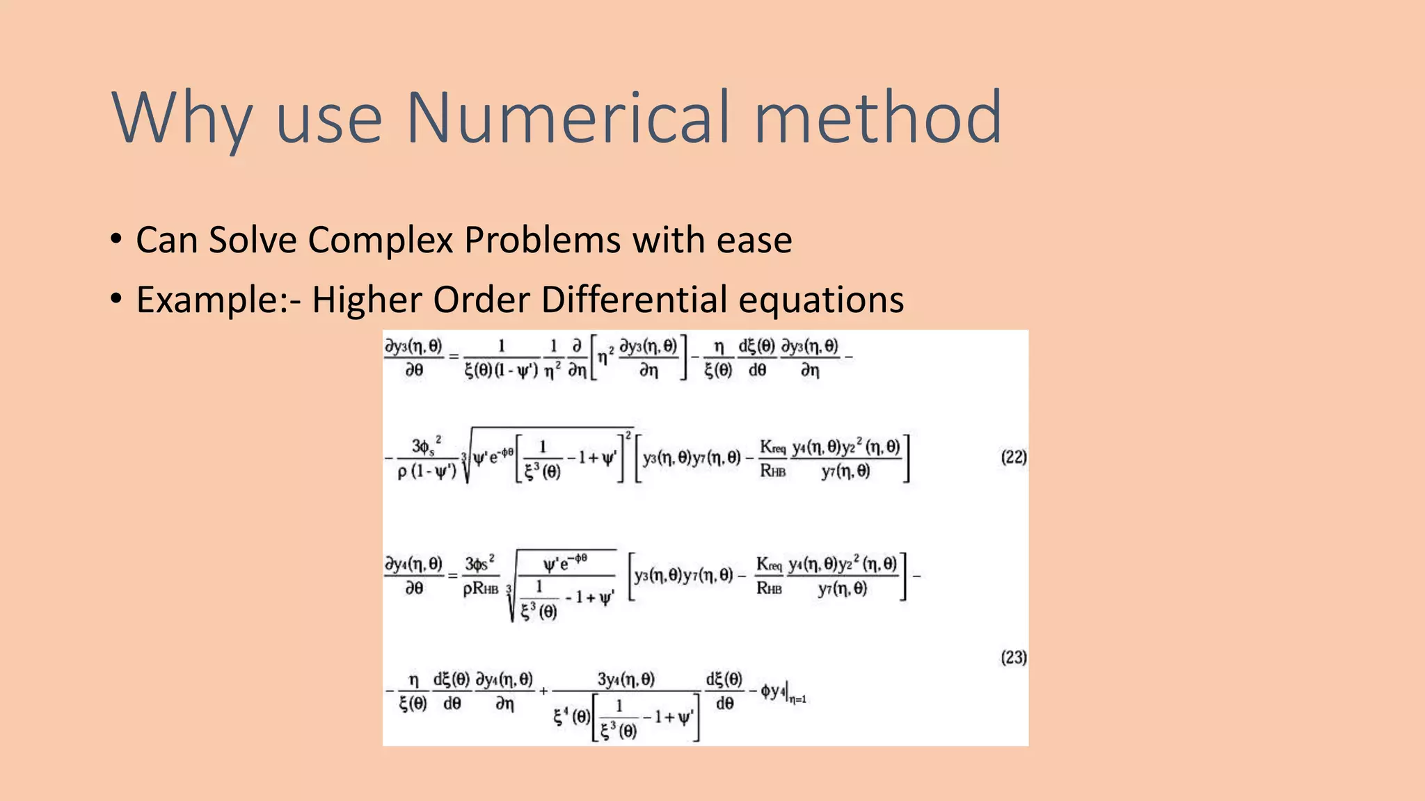
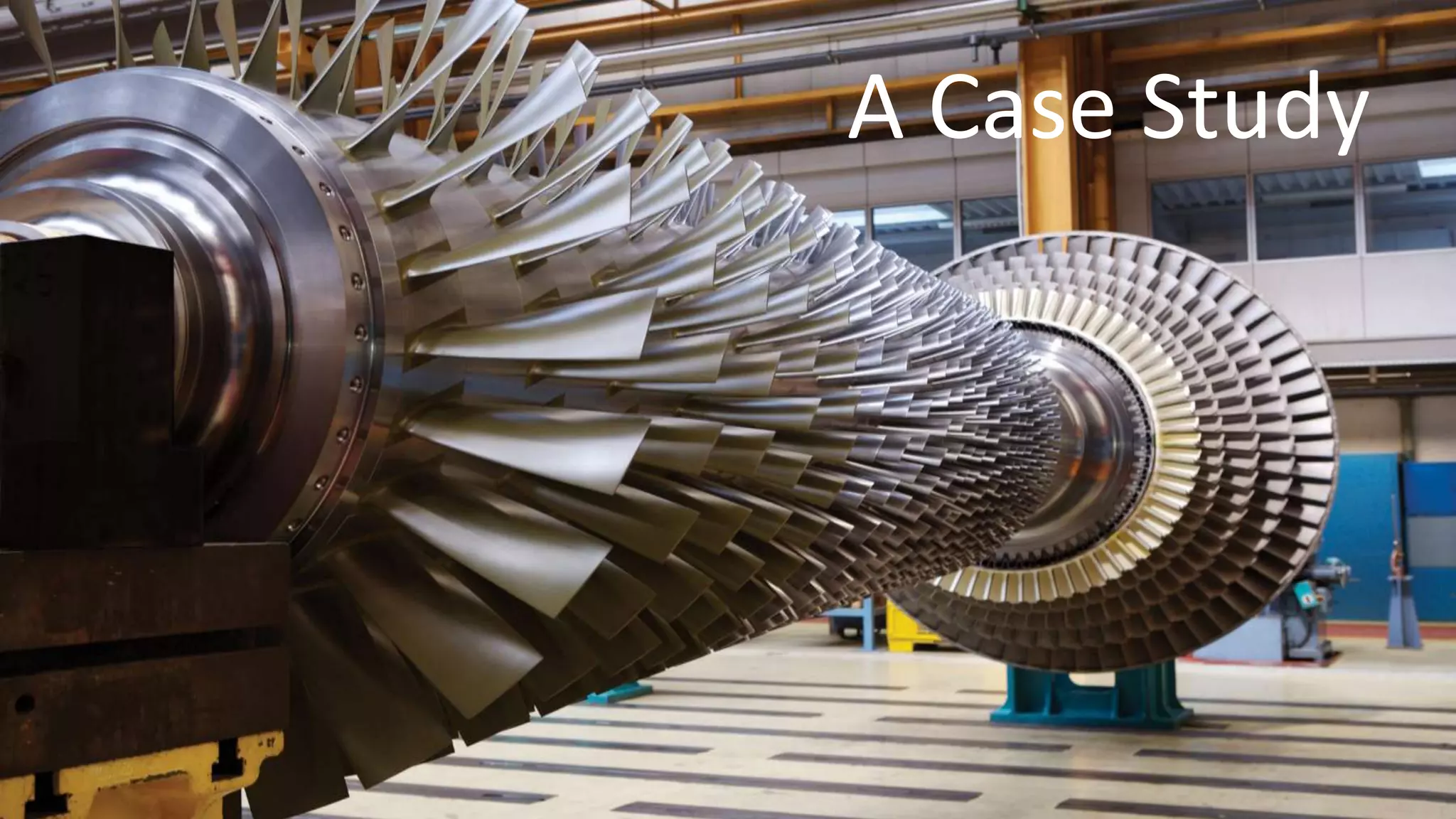
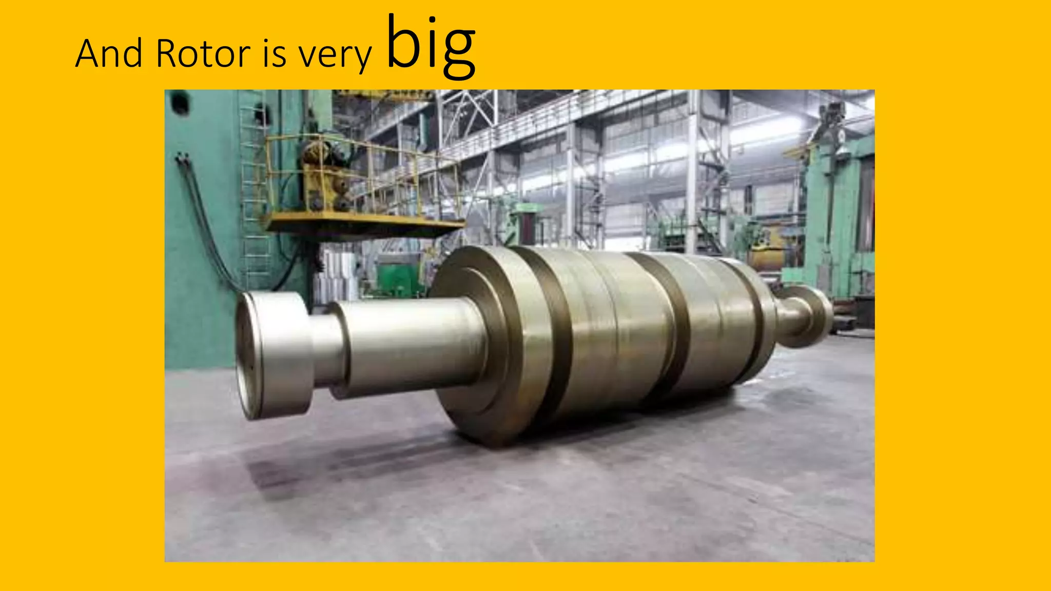
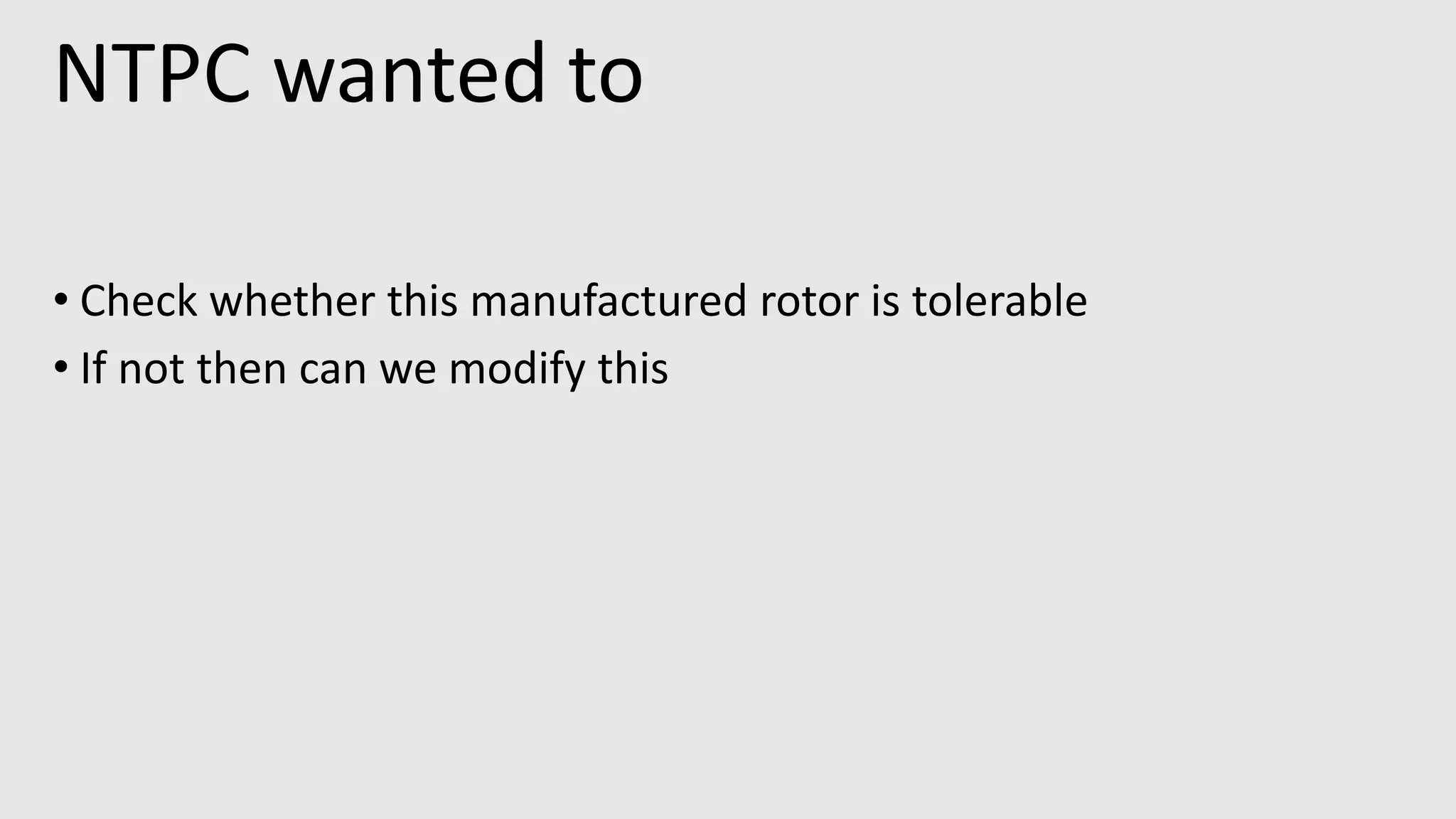
The document provides an introduction to finite element analysis. It discusses the need for computational methods to solve problems involving complex geometries and boundary conditions that cannot be solved through closed-form analytical methods. The finite element method is introduced as a numerical technique that involves discretizing a continuous domain into discrete subdomains called elements, and approximating variations in dependent variables within each element. This allows setting up algebraic equations that can be solved to approximate the continuous solution. Advantages of the finite element method include its ability to model complex shapes and behaviors, and refine solutions through mesh refinement. Basic concepts such as element types, discretization, and derivation of element equations are described.
The document discusses various numerical methods for analyzing mechanical components under applied loads, including the finite element method. It describes weighted residual methods like the Galerkin method and collocation method which approximate solutions by minimizing residuals. The variational or Rayleigh-Ritz method selects displacement fields to minimize total potential energy. The finite element method divides a structure into small elements and applies these methods to obtain approximate solutions for displacements and stresses at discrete points.
What is a multiple dgree of freedom (MDOF) system?
How to calculate the natural frequencies?
What is a mode shape?
What is the dynamic stiffness matrix approach?
#WikiCourses
https://wikicourses.wikispaces.com/Lect04+Multiple+Degree+of+Freedom+Systems
https://eau-esa.wikispaces.com/Topic+Multiple+Degree+of+Freedom+%28MDOF%29+Systems
Finite element method vs classical method 1manoj kumar
The document provides an introduction to the finite element method. It compares the finite element method to classical methods and the finite difference method. Some key differences highlighted include:
- Classical methods obtain exact solutions for simple cases while finite element methods obtain approximate solutions for all problems.
- Finite element methods can handle problems with complex geometry, multi-materials, and non-linearities, while classical methods have difficulties with these.
- Finite difference methods make point-wise approximations while finite element methods make piece-wise approximations, allowing for continuity along element boundaries.
- Finite element methods can evaluate values between nodes through interpolation, while finite difference methods only provide values at nodes.
The document provides an introduction to the finite element method (FEM). It discusses that FEM is a numerical technique used to approximate solutions to boundary value problems defined by partial differential equations. It can handle complex geometries, loadings, and material properties that have no analytical solution. The document outlines the historical development of FEM and describes different numerical methods like the finite difference method, variational method, and weighted residual methods that FEM evolved from. It also discusses key concepts in FEM like discretization into elements, node points, and interpolation functions.
This document provides an overview of a course on engineering design and rapid prototyping. It discusses the finite element method (FEM) which will be covered in class. FEM involves cutting a structure into small elements and connecting them at nodes to form algebraic equations that can be solved numerically. This allows for approximate solutions to complex problems. The document outlines the typical FEM procedure of preprocessing, analysis, and postprocessing using software. It also discusses sources of errors in the FEM approach and mistakes users may make.
The document discusses numerical methods for solving structural mechanics problems, specifically the Rayleigh Ritz method. It provides an overview of the Rayleigh Ritz method, indicating that it is an integral approach that is useful for solving structural mechanics problems. The document then provides a step-by-step example of using the Rayleigh Ritz method to determine the bending moment and deflection at the mid-span of a simply supported beam subjected to a uniformly distributed load over the entire span.
The document provides an overview of the finite element method (FEM). It explains that FEM is a numerical technique used to approximate solutions to partial differential equations that describe physical phenomena. It works by dividing a complex geometry into small pieces called finite elements that can then be solved using a computer. The method was developed in the 1950s and has since become widely used in engineering fields to simulate systems like heat transfer, stress analysis, and fluid flow. The document outlines the basic approach of FEM and traces the history and development of its early software programs.
This document summarizes a finite element analysis of a cantilever beam using quadrilateral meshing elements. The beam is modeled and analyzed in Abaqus for three loading cases: a point load at the free end, a point load at the mid-section, and a distributed load along the length. Hand calculations are also performed and compared to Abaqus and MATLAB results. Increasing the number of elements improves accuracy of the models. Quadrilateral elements are preferred over triangular elements for beam bending problems. Maximum displacement occurs under a point load at the free end. The study concludes with recommendations for accurate beam modeling and design using finite element analysis.
FEM: Introduction and Weighted Residual MethodsMohammad Tawfik
What are weighted residual methods?
How to apply Galerkin Method to the finite element model?
#WikiCourses #Num001
https://wikicourses.wikispaces.com/TopicX+Approximate+Methods+-+Weighted+Residual+Methods
- The document discusses one-dimensional finite element analysis.
- It describes the derivation of shape functions for linear one-dimensional elements like a bar element. Shape functions define the variation of displacement within the element.
- The stiffness matrix, which represents the element's resistance to deformation, is also derived for a basic linear bar element. It is shown to be symmetric and its properties are discussed.
- Examples are provided to demonstrate calculating displacements at points within a one-dimensional element using the shape functions.
The document discusses the finite element method (FEM) for analyzing beam structures. FEM involves subdividing a structure into finite elements of simple shape and solving for the whole structure. Elements can be one-, two-, or three-dimensional, with accuracy increasing with more elements. Nodes are points where elements connect, and nodal displacements describe element deformation. FEM allows analyzing complex shapes like plates by treating them as assemblies of beams. A simple bar analysis example demonstrates deriving and solving the stiffness matrix to determine displacements and forces from applied loads.
This document discusses two-dimensional vector variable problems in structural mechanics. It describes plane stress, plane strain and axisymmetric problems, and provides the stress-strain relations for materials under these conditions. It also discusses thin structures like disks and long prismatic shafts. Additionally, it covers dynamic analysis and vibration of structures, describing free vibration, forced vibration and types of vibration. Equations of motion are developed using Lagrange's approach and the weak form method. Mass and stiffness matrices for axial rod and beam elements are also presented.
The finite element method is used to solve engineering problems involving stress analysis, heat transfer, and other fields. It involves dividing a structure into small pieces called finite elements and deriving the governing equations for each element. The element equations are assembled into a global stiffness matrix and force vector. Boundary conditions are applied and the system is solved for the unknown displacements at nodes. Results like stresses, strains, and temperatures are then determined. Key steps are discretization, deriving the element stiffness matrix, assembling the global matrix, applying boundary conditions, and solving for nodal displacements.
This document provides an overview of finite element analysis (FEA). It defines FEA as a numerical method for solving governing equations over the domain of a continuous physical system that is discretized into simple shapes. It lists several common structural and non-structural applications of FEA, such as stress analysis, buckling problems, vibration analysis, and heat transfer. Finally, it provides the course outline, textbooks, references, and some common FEA software packages.
This document provides an overview of a course on the finite element method. The course objectives are for students to learn how to write simple programs to solve problems using FEM. Assessment includes assignments, quizzes, a course project, midterm exam, and final exam. Fundamental agreements include electronic homework submission and using MATLAB or Mathematica. References on FEM are also provided. The document outlines numerical methods for solving boundary value problems and introduces weighted residual methods like the collocation method, subdomain method, and Galerkin method.
single degree of freedom systems forced vibrations KESHAV
SDOF, Forced vibration
includes following content
Forced vibrations of longitudinal and torsional systems,
Frequency Response to harmonic excitation,
excitation due to rotating and reciprocating unbalance,
base excitation, magnification factor,
Force and Motion transmissibility,
Quality Factor.
Half power bandwidth method,
Critical speed of shaft having single rotor of undamped systems.
This document provides an overview of the finite element method (FEM) for a course on engineering geology. It outlines the course content, which includes an introduction to FEM, the Ritz-Galerkin and weak form methods, and applying FEM to 1D and 2D problems. Key aspects of FEM discussed include reducing partial differential equations to a system of algebraic equations, dividing problems into finite elements, and constructing approximate functions and element matrices. The origins and importance of FEM for solving complex problems are also summarized.
The document discusses isoparametric finite elements. It defines isoparametric, superparametric, and subparametric elements. It provides examples of shape functions for 4-noded rectangular, 6-noded triangular, and 8-noded rectangular isoparametric elements. It also discusses coordinate transformation from the natural to global coordinate system using these shape functions and calculating the Jacobian.
Introduction to finite element analysisTarun Gehlot
The document provides an introduction to finite element analysis (FEA) or the finite element method (FEM). It describes FEA as a numerical method used to solve engineering and mathematical physics problems that cannot be solved through analytical methods due to complex geometries, loadings, or material properties. FEA involves discretizing a complex model into smaller, simpler elements connected at nodes, then applying the governing equations to obtain a numerical solution for the unknown primary variable (usually displacement) at nodes. Secondary variables like stress are then determined from nodal displacements. The process involves preprocessing, solving, and postprocessing steps.
The document discusses two-dimensional finite element analysis. It describes triangular and quadrilateral elements used for 2D problems. The derivation of the stiffness matrix is shown for a three-noded triangular element. Shape functions are presented for triangular and quadrilateral elements. Examples are provided to calculate strains for a triangular element and to determine temperatures at interior points using shape functions.
FEM is about to Finite element method. In this it is described that how FEM is done and what are the steps which we have to follow for fully FEA. Finite Element Analysis is one of the most important analysis which is used in various field.
This document provides an overview of ANSYS Workbench software for structural and thermal analysis. It describes the user interface, types of analysis available including linear static, modal, heat transfer and buckling. It outlines the steps to set up a static structural analysis including importing geometry, applying materials, meshing, boundary conditions and solving. License types are also summarized. The goal is to teach the basics of using simulation capabilities in ANSYS Workbench.
This document provides an introduction and overview to using ANSYS Mechanical within the ANSYS Workbench environment. It outlines the objectives and agenda for a two-day training course covering topics such as importing geometry, meshing, applying loads and boundary conditions, and post-processing results. It also provides information on the ANSYS Workbench interface, including the toolbox, project schematic, and file management.
The Finite Element Method (FEM) is a numerical technique for solving problems of engineering and mathematical physics. It subdivides a large problem into smaller, simpler parts that are called finite elements. FEM allows for complex geometries and loading conditions to be modeled. The process involves discretizing the domain into elements, deriving the governing equations for each element, assembling the element equations into a global system of equations, and solving the system to obtain the unknown variable values. FEM can handle a wide range of problems including nonlinear problems and transient problems.
The document introduces the finite element method (FEM). It defines FEM as a numerical method used to solve mechanical engineering problems. It discusses the key steps and types of elements in FEM. The pre-processing step involves discretization or meshing. The solution process involves determining the local and global stiffness matrices. The post-processing step analyzes the results. It also describes the different types of forces (body, surface, point) and elements (1D, 2D, 3D) used in FEM.
This document provides an overview of the finite element method (FEM). It discusses the potential energy approach, discretization, boundary conditions, strain-displacement relationships, stress-strain behaviors, element and global stiffness matrices, and solution schemes for structural analysis problems. It also covers FEM terminology and concepts such as nodes, elements, and iterative methods for solving systems of linear equations. Finally, it notes some limitations of the FEM.
The document outlines a 16-week course on the finite element method (FEM). It introduces FEM and its applications in heat transfer, fluid mechanics, and solid mechanics. Over the course, students will learn how to formulate the finite element equation, create elements to model problems, and solve problems using FEM software. Assessment includes homework, programming tests, a midterm, and a final exam.
1. The charge simulation method (CSM) simulates an actual electric field with a field formed by discrete charges placed outside the region where the field solution is desired.
2. CSM determines the values of discrete charges by satisfying boundary conditions at selected contour points on electrodes. Once charge values and positions are known, the potential and field distribution can be easily computed.
3. CSM describes surface charge on an electrode boundary using fictitious point, line, or ring charges in the electrode interior. Charge types and positions are determined first, then magnitudes are calculated to satisfy boundary conditions.
The document provides an overview of the history and basics of finite element analysis (FEA). It discusses how FEA was first developed in 1943 and expanded in the following decades. The basics section describes common FEA applications, basic steps which include converting differential equations to algebraic equations, element types, boundary conditions including loads and constraints, and pre-processing, solving, and post-processing steps. Key element types are also summarized.
The document provides an introduction to the finite element method (FEM) by comparing it to the finite difference method (FDM) in solving a steady state heat conduction problem. It explains key FEM concepts like weighted residuals, interpolation functions, numerical integration using Gauss quadrature, and applying essential boundary conditions. Examples are presented to illustrate the standard FEM procedure of developing element stiffness matrices, applying nodal connectivity, and assembling the global matrix to obtain a numerical solution.
INTRODUCTION TO FINITE ELEMENT ANALYSISAchyuth Peri
Finite element analysis (FEA) is a numerical technique used to find approximate solutions to partial differential equations. It involves dividing a system into small elements and solving for variables within each element. This allows for analysis of complex geometries, loadings, and materials. The FEM process includes discretizing the system, selecting functions to approximate the solution, assembling element equations into a global system, applying boundary conditions, and calculating displacements, stresses, and strains. FEA offers advantages like analyzing irregular shapes and nonlinear problems, reducing testing costs, and optimizing designs.
FEA Basic Introduction Training By Praveenpraveenpat
Finite Element Analysis (FEA) involves discretizing a structure into small pieces (elements) and using a mathematical model to simulate loads and stresses on the structure. The key steps are: 1) Discretizing the structure into elements, 2) Developing element equations, 3) Assembling equations into a global system, 4) Applying boundary conditions, 5) Solving for unknowns, and 6) Calculating derived variables like stresses and displacements. FEA is commonly used in engineering fields like automotive, aerospace, and mechanical engineering to analyze stresses, deflections, and other performance aspects of complex structures.
This document summarizes a finite element study of piezoelectric thin films on substrates. It outlines the background on piezoelectricity, modeling preliminaries including governing equations and material properties. It then lists the main tasks which include analyzing the effects of periodicity, lattice mismatch, and different film-substrate properties on the piezoelectric response and internal stress. Publications resulting from this work are also listed.
07 a70102 finite element methods in civil engineeringimaduddin91
This document contains 8 questions related to the finite element method in civil engineering. The questions cover various topics including:
1) Deriving expressions for potential energy and determining displacements using Rayleigh Ritz method for a 1D rod subjected to loading.
2) Assembling stiffness and force matrices and determining displacements and stresses for a 1D rod under thermal loading using finite element discretization.
3) Evaluating shape functions and determining the Jacobian for an isoparametric triangular element.
The document provides figures and equations to accompany the questions. It examines a range of finite element techniques including shape function derivation, element formulation, structural and thermal analysis, and plate bending elements.
Townsend ’s theory
Introduction
Ionization by collision
Townsend’s current growth equation
Current Growth in the Presence of Secondary Processes
Townsend’s secondary ionization coefficient
Townsend’s Criterion for Breakdown
Breakdown in Electronegative Gases
1. The document describes a finite difference element method for modeling paper response using the software FLAC.
2. Key aspects of the method include assigning local material properties and constitutive relationships to each element based on spatial variations in paper properties like basis weight and fiber orientation.
3. The model will be verified by comparing predictions of energy dissipation during inelastic deformation to infrared camera measurements with high resolution, and relating the evolution of inelastic zones to measured basis weight maps.
410102 Finite Element Methods In Civil Engineeringguestac67362
This document contains a sample exam for a Finite Element Methods in Civil Engineering course. It lists 8 questions related to finite element analysis concepts and applications. Students must answer 5 of the 8 questions, which cover topics such as derivation of stiffness matrices, strain-displacement relationships, shape functions, axisymmetric problems, and numerical integration techniques. Solutions are provided for planar structures, beams, trusses, and other structural elements.
The document summarizes the finite difference method (FDM) for vibration analysis of beams. FDM is an approximate method that involves dividing the continuum of a beam into a mesh and expressing the differential equation governing beam vibration as a set of finite difference equations at each node. As an example, a beam is divided into four segments and the resulting finite difference equations representing the boundary conditions and governing differential equation are solved as an eigenvalue problem to determine the fundamental natural frequency and first mode shape of the beam.
This document discusses heat transfer through conduction and various methods for solving the heat equation using finite difference approximations. It introduces the heat equation in Cartesian, cylindrical and spherical coordinates. It discusses boundary conditions and describes setting up a nodal network to discretize the domain. It then presents the finite difference form of the heat equation and describes different cases for nodal finite difference equations, including for interior nodes, nodes at corners or surfaces with convection, and nodes at surfaces with uniform heat flux. It discusses solving the finite difference equations using matrix inversion, Gauss-Seidel iteration, and provides examples.
This document summarizes a student project that used the finite difference method and the Laplace equation to model the electrostatic properties of a non-symmetrical surface. The student created an Excel model of an infinitely long magnetic strip surrounded by a conducting box. The model was used to calculate potential, electric field, surface charge density, and capacitance per unit length for different node amounts. The results showed higher potential and charge density near the strip, and flux lines directed towards the box edges rather than another plate. Overall, the model behaved similarly to a parallel-plate capacitor except for non-symmetrical flux lines.
The electric force between two charged particles is:
- Inversely proportional to the square of the distance between them
- Directed along the line joining the particles
- Attractive if charges have opposite signs, repulsive if the same
The electric field E at a point is defined as the electric force on a positive test charge at that point divided by the magnitude of the test charge. Electric field lines are drawn tangent to the field, with a higher density of lines indicating a greater field magnitude.
Optimal Finite-Difference Grids for Elliptic Problem
In many applications one observes rapid change of the solution in the boundary region. Accurate and numerically efficient resolution of the solution close to the moving boundaries is considered to be and important problem. We develop an approach to grid optimization for finite-difference scheme for elliptic problem. Using this approach we are able to achieve exponential convergence of the boundary Neumann-to-Dirichlet map when applied to the bounded domains. It increases the convergence order without increasing the stencil size of the finite-difference scheme and without losing stability.
The document discusses finite element methods and their applications in microelectromechanical systems (MEMS). It covers the basic formulation of finite element methods, including discretization, selection of displacement functions, derivation of element stiffness matrices, and assembly of global equations. It also discusses specific applications of finite element analysis to problems in MEMS like heat transfer analysis, thermal stress analysis, and static/modal analysis. The finite element method is well-suited for complex geometries and materials and can model irregular shapes, general loads/boundary conditions, and nonlinear behavior.
This document discusses finite element analysis and nonlinear finite element analysis. It introduces the finite element method and how it approximates solutions by dividing them into discrete elements. It explains that higher order polynomials and more nodes/elements increase accuracy. The document distinguishes between linear and nonlinear problems, with nonlinear problems not obeying Hooke's law. It lists common finite element methods for nonlinear mechanics like updated Lagrangian formulations. Finally, it discusses solution algorithms for nonlinear problems like Newton's method and line searches.
This document provides an overview of a course on the finite element method for analyzing linear systems taught at the Swiss Federal Institute of Technology. The first lecture covers the motivation and organization of the course, introduces the use of finite elements by relating physical problems to mathematical modeling and finite element solutions, and discusses basic mathematical tools used in finite element analysis like vectors, matrices, and tensors.
Operational research models can help organizations in various sectors. Some key examples include:
1) British Telecom used an OR model to schedule over 40,000 field engineers, saving $150 million annually from 1997-2000.
2) Continental Airlines developed a crew scheduling model to help resume normal operations just days after 9/11.
3) Ford Motor Company reduced annual prototype costs by $250 million using an optimization model to share prototype vehicles between testing needs.
This document discusses improving the simplicity of use of constraint programming (CP) for industrial applications. It argues that while CP can achieve good performance, it is difficult for engineers to learn, use, and maintain due to its complexity. The CP academic community focuses on adding new modeling features and techniques rather than usability, making CP even more complex over time. The document recommends that the CP community learn from the mathematical programming (MP) and SAT communities, which provide better out-of-the-box performance and usability. Specific recommendations include standardizing modeling languages and formats, improving search algorithms, adding explanations and optimization capabilities, and focusing on modeling practices and benchmarking running times.
This is a little presentation I gave to Roald Hoffmann's group at Cornell. What are the industrial applications of computational chemistry? How to people work differently in academia vs. industry? What are the sorts of things students should think about if they plan to work in the corporate world?
Optimization techniques are used to find the best formulation and manufacturing process. Traditional optimization varies one variable at a time, while modern techniques use systematic experimental design. Different optimization methods are applied depending on the problem, such as whether the problem has constraints or independent variables. Optimization helps reduce costs and errors while improving safety, reproducibility, and time efficiency in pharmaceutical development and manufacturing.
Unit I fdocuments.in_introduction-to-fea-and-applications.pptAdityaChavan99
The document provides an introduction to finite element analysis (FEA) and its applications to engineering problems. It discusses that FEA is a numerical method used to solve problems that cannot be solved analytically due to complex geometry or materials. It involves discretizing a continuous structure into small, well-defined substructures called finite elements. The key steps in FEA include preprocessing such as defining geometry, meshing and material properties, solving the problem, and postprocessing results such as stresses and strains. The document also discusses various element types, assembly of elements, sources of error in FEA, and its advantages such as handling complex geometry, loading and materials.
Operation research history and overview application limitationBalaji P
This document provides an overview of operation research (OR). It discusses OR topics like quantitative approaches to decision making, the history and definition of OR, common OR models like linear programming and network flow programming, and applications of OR. It also explains problem solving, decision making, and quantitative analysis approaches. OR aims to apply analytical methods to help make optimal decisions for complex systems and problems.
The document provides an introduction to finite element analysis (FEA) including:
1) FEA involves discretizing a continuous structure into small substructures called finite elements connected at nodes. This process is called meshing.
2) The finite element method has three main phases - preprocessing (defining geometry, materials, mesh), solution (solving equations to obtain nodal results), and postprocessing (obtaining stresses, strains from nodal results).
3) FEA can model complex problems that cannot be solved analytically due to complicated geometry or materials, and is well-suited for solving problems in solid mechanics, heat transfer, and other fields on computers.
'A critique of testing' UK TMF forum January 2015 Georgina Tilby
This presentation draws upon the 'Critique of Testing' Ebook that was discussed at January's UK TMF forum. The slides explore the fundamental concepts of test case design and provide a detailed analysis of each method in terms of them.
Planning of experiment in industrial researchpbbharate
This document discusses key concepts in the design of experiments. It begins with definitions of systems and processes, and defines an experiment as a test where input variables are deliberately changed to observe their effects on outputs. The objectives of experiments are identified as understanding factor effects and developing models. Basic principles for experimental design are outlined, including randomization, replication, and blocking. Guidelines are provided for various steps in designing an experiment, from problem definition to statistical analysis and conclusions. Examples are given throughout to illustrate experimental design concepts.
The document discusses introducing mixed effects models. It focuses on fixed effects, which are the effects of interest. This week covers sample datasets, theoretical models, fitting models in R, and interpreting parameters like slopes and intercepts. The sample dataset examines factors like newcomers and experience that influence how long teams take to assemble phones. The document uses this example to demonstrate key steps in modeling fixed effects, such as estimating slopes, intercepts, and conducting hypothesis tests on parameters.
Lecture 1 Chapter 1 Introduction to OR.pdfVamshi962726
This document provides information about an Operations Research course. It includes:
1) General course information such as the instructor's name and contact details, course credits, prerequisites, textbook, and course description.
2) An overview of topics to be covered including modeling with linear programming, the simplex method, transportation models, and network models.
3) Course objectives, expectations for written assignments, class rules, policies on attendance and cell phone use, and the course assessment breakdown.
4) A description of the course project involving application of the cutting stock problem to a real-life setting.
5) An introduction to operations research including its origins, applications, approach involving defining problems and constructing mathematical models
Writing for computer science: Fourteen steps to a clearly written technical p...aftab alam
The document outlines 14 steps for writing a clearly written technical paper, including:
1. Complete the first draft except for the introduction and conclusion.
2. Organize ideas in the correct order so each section logically follows from the previous.
3. Use transitions between ideas to guide the reader.
4. Ensure each paragraph has a single main point stated in the first sentence.
5. Simplify sentences and reduce abstract words to improve clarity and readability.
A Survey on Automatic Software Evolution TechniquesSung Kim
The document discusses automatic software evolution techniques. It describes approaches like refactoring, automatic patch generation, runtime recovery and performance improvement. The most popular current approach is "generate and validate" which evolves a program with validation. Challenges include search space explosion as techniques are limited in the variants they can generate, and developing effective search methods to find valid patches. The document proposes mining existing software changes to learn common templates to guide the search for valid patches.
Lecture on Introduction to finite element methods & its contentsMesayAlemuTolcha1
The document provides an overview of the Finite Element Method (FEM) course being taught. It discusses:
1. What FEM is and its common application areas like structural analysis, heat transfer, fluid flow.
2. The main steps in FEM including discretization, selecting interpolation functions, developing element matrices, assembling the global matrix, imposing boundary conditions, and solving equations.
3. Different element types like 1D, 2D, and 3D elements and the use of isoparametric formulations.
4. The history of FEM and how it has evolved from being used on mainframe computers to PCs.
The document provides examples and explanations of key concepts in problem solving and algorithms:
1) It defines problem analysis as understanding the problem by identifying the 5 Ws (what, who, when, where, why), and provides two examples of problem analysis.
2) It defines an algorithm as a set of steps to accomplish a task, and explains their role and importance in problem solving through examples.
3) It discusses how to choose the most efficient algorithm when multiple algorithms exist to solve a problem, using examples to compare efficiency based on steps and memory usage.
This document discusses various problem solving tools and techniques. It begins by describing the importance of root cause problem solving over simply treating symptoms. It then discusses different problem solving tools like 5 whys, logic trees, and 7 step problem solving and how to select the appropriate tool based on the situation. It provides examples of each tool. The key takeaways are that the level of complexity will determine the best tool, and many problems can be solved quickly with root cause analysis or 5 whys. Logic trees are useful for organizing problem solving efforts.
Concept Location using Information Retrieval and Relevance FeedbackSonia Haiduc
Concept location is a critical activity during
software evolution as it produces the location where a change is to start in response to a modification
request, such as, a bug report or a new feature request. Lexical-based concept location techniques rely on matching the text embedded in the source code to queries formulated by the developers. The efficiency of such techniques is strongly dependent on the ability of the developer to write good queries. We propose an approach to augment information retrieval (IR) based concept location via an explicit relevance feedback (RF) mechanism. RF is a two-part process in which the developer judges existing results returned by a search and the IR system uses this information to perform a new search, returning more relevant information to the user. A set of case studies performed on open source software systems reveals the impact of RF on IR based concept location.
This document presents a study on using relevance feedback to improve information retrieval-based concept location in software engineering. The study uses an IR tool with the Lucene engine and Rocchio algorithm for relevance feedback. It evaluates the tool on bug reports from Eclipse, jEdit, and Adempiere, measuring the number of methods investigated before finding the target method with and without relevance feedback. The results show relevance feedback improved concept location in most cases by reformulating queries based on developer feedback on result relevancy. Future work includes more experiments and automatically calibrating parameters.
UNIT-2 Quantitaitive Anlaysis for Mgt Decisions.pptxMinilikDerseh1
This document provides an overview of linear programming problems (LPP). It discusses the key components of linear programming models including objectives, decision variables, constraints, and parameters. It also covers formulation of LPP, graphical and simplex solution methods, duality, and post-optimality analysis. Various applications of linear programming in areas like production, marketing, finance, and personnel management are also highlighted. An example problem on determining optimal product mix given resource constraints is presented to illustrate linear programming formulation.
Advanced control scheme of doubly fed induction generator for wind turbine us...IJECEIAES
This paper describes a speed control device for generating electrical energy on an electricity network based on the doubly fed induction generator (DFIG) used for wind power conversion systems. At first, a double-fed induction generator model was constructed. A control law is formulated to govern the flow of energy between the stator of a DFIG and the energy network using three types of controllers: proportional integral (PI), sliding mode controller (SMC) and second order sliding mode controller (SOSMC). Their different results in terms of power reference tracking, reaction to unexpected speed fluctuations, sensitivity to perturbations, and resilience against machine parameter alterations are compared. MATLAB/Simulink was used to conduct the simulations for the preceding study. Multiple simulations have shown very satisfying results, and the investigations demonstrate the efficacy and power-enhancing capabilities of the suggested control system.
Electric vehicle and photovoltaic advanced roles in enhancing the financial p...IJECEIAES
Climate change's impact on the planet forced the United Nations and governments to promote green energies and electric transportation. The deployments of photovoltaic (PV) and electric vehicle (EV) systems gained stronger momentum due to their numerous advantages over fossil fuel types. The advantages go beyond sustainability to reach financial support and stability. The work in this paper introduces the hybrid system between PV and EV to support industrial and commercial plants. This paper covers the theoretical framework of the proposed hybrid system including the required equation to complete the cost analysis when PV and EV are present. In addition, the proposed design diagram which sets the priorities and requirements of the system is presented. The proposed approach allows setup to advance their power stability, especially during power outages. The presented information supports researchers and plant owners to complete the necessary analysis while promoting the deployment of clean energy. The result of a case study that represents a dairy milk farmer supports the theoretical works and highlights its advanced benefits to existing plants. The short return on investment of the proposed approach supports the paper's novelty approach for the sustainable electrical system. In addition, the proposed system allows for an isolated power setup without the need for a transmission line which enhances the safety of the electrical network
Null Bangalore | Pentesters Approach to AWS IAMDivyanshu
#Abstract:
- Learn more about the real-world methods for auditing AWS IAM (Identity and Access Management) as a pentester. So let us proceed with a brief discussion of IAM as well as some typical misconfigurations and their potential exploits in order to reinforce the understanding of IAM security best practices.
- Gain actionable insights into AWS IAM policies and roles, using hands on approach.
#Prerequisites:
- Basic understanding of AWS services and architecture
- Familiarity with cloud security concepts
- Experience using the AWS Management Console or AWS CLI.
- For hands on lab create account on [killercoda.com](https://killercoda.com/cloudsecurity-scenario/)
# Scenario Covered:
- Basics of IAM in AWS
- Implementing IAM Policies with Least Privilege to Manage S3 Bucket
- Objective: Create an S3 bucket with least privilege IAM policy and validate access.
- Steps:
- Create S3 bucket.
- Attach least privilege policy to IAM user.
- Validate access.
- Exploiting IAM PassRole Misconfiguration
-Allows a user to pass a specific IAM role to an AWS service (ec2), typically used for service access delegation. Then exploit PassRole Misconfiguration granting unauthorized access to sensitive resources.
- Objective: Demonstrate how a PassRole misconfiguration can grant unauthorized access.
- Steps:
- Allow user to pass IAM role to EC2.
- Exploit misconfiguration for unauthorized access.
- Access sensitive resources.
- Exploiting IAM AssumeRole Misconfiguration with Overly Permissive Role
- An overly permissive IAM role configuration can lead to privilege escalation by creating a role with administrative privileges and allow a user to assume this role.
- Objective: Show how overly permissive IAM roles can lead to privilege escalation.
- Steps:
- Create role with administrative privileges.
- Allow user to assume the role.
- Perform administrative actions.
- Differentiation between PassRole vs AssumeRole
Try at [killercoda.com](https://killercoda.com/cloudsecurity-scenario/)
Comparative analysis between traditional aquaponics and reconstructed aquapon...bijceesjournal
The aquaponic system of planting is a method that does not require soil usage. It is a method that only needs water, fish, lava rocks (a substitute for soil), and plants. Aquaponic systems are sustainable and environmentally friendly. Its use not only helps to plant in small spaces but also helps reduce artificial chemical use and minimizes excess water use, as aquaponics consumes 90% less water than soil-based gardening. The study applied a descriptive and experimental design to assess and compare conventional and reconstructed aquaponic methods for reproducing tomatoes. The researchers created an observation checklist to determine the significant factors of the study. The study aims to determine the significant difference between traditional aquaponics and reconstructed aquaponics systems propagating tomatoes in terms of height, weight, girth, and number of fruits. The reconstructed aquaponics system’s higher growth yield results in a much more nourished crop than the traditional aquaponics system. It is superior in its number of fruits, height, weight, and girth measurement. Moreover, the reconstructed aquaponics system is proven to eliminate all the hindrances present in the traditional aquaponics system, which are overcrowding of fish, algae growth, pest problems, contaminated water, and dead fish.
1. JK Lakshmipat University
Institute of Engineering and technology
Finite Element Method
Submitted to:
Prof R.K. Agrawal
Submitted by:
Bharat Sharma
2012BTechME008
3. Analytical Methods V/S
Numerical Methods
Find the root of f(x)=x−5
Analytical solution: f(x)=x−5=0
add +5 to both sides to get the answer x=5
Numerical solution:
Let's guess x=1: f(1)=1−5=−4. A negative number.
Let's guess x=6: f(6)=6−5= 1. A positive number.
And you get a range in which solution exists.
4. Why use Numerical method
• Can Solve Complex Problems with ease
• Example:- Higher Order Differential equations
5. Why use Analytical Method
• To validate results from Numerical Methods
• Analytical solutions can be obtained exactly with pencil and paper
6. What is FEM ?
• Finite Element Method
• A type of Numerical Method
• Used for solving a differential or integral equation.
• It has been applied to a number of physical problems, where the
governing differential equations are available.
8. Area of geometry = A1 + A2 + A3 – A4
1
2
3
4
Finite Element method
It is not of course used to calculate areas, but
things like displacements, temperatures,
velocities, stresses and so on
Meshing
9. Is FVM related to FEM
• Finite volumetric method
• 3D version of FEM
• Most of the commercial analysis software work on the principle of
FVM
11. Stress Analysis of LP Rotor
Problem:-
• To determine stresses in the existing rotor
• To modify the defective Rotor geometry and limit the stress to the existing
value
Client : N.T.P.C. New Delhi Done by : IIT Madras
12. You can see that there is a small hole there. The
problem is that this small hole or defect which
has been created due to improper
manufacturing, it so happens that it is at a
place where the stresses are also high
13. Can’t you just manufacture another ?
• Rotor is very expensive, it is about 10 crores
• Lead time to manufacture this rotor is nearly 6 months
• A particular thermal power project worth about 3000 crores is going
to stand still.