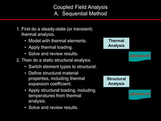
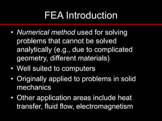
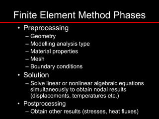
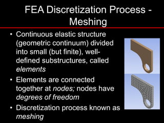
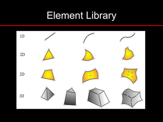
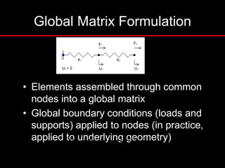
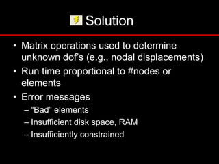
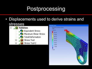
The document provides an introduction to finite element analysis (FEA) and its applications to engineering problems. It discusses that FEA is a numerical method used to solve problems that cannot be solved analytically due to complex geometry or materials. It involves discretizing a continuous structure into small, well-defined substructures called finite elements. The key steps in FEA include preprocessing such as defining geometry, meshing and material properties, solving the problem, and postprocessing results such as stresses and strains. The document also discusses various element types, assembly of elements, sources of error in FEA, and its advantages such as handling complex geometry, loading and materials.

1. Introduction to Design with Finite Element
Approach and Applications to Engineering
Problems
Dr. K. Padmanabhan FIIPE, FIE, CE(I),FISME
Professor
Manufacturing Division
School of MBS
VIT-University
Vellore 632014
February 2013

2. FEA Introduction
• Numerical method used for solving
problems that cannot be solved
analytically (e.g., due to complicated
geometry, different materials)
• Well suited to computers
• Originally applied to problems in solid
mechanics
• Other application areas include heat
transfer, fluid flow, electromagnetism

3. Finite Element Method Phases
• Preprocessing
– Geometry
– Modelling analysis type
– Material properties
– Mesh
– Boundary conditions
• Solution
– Solve linear or nonlinear algebraic equations
simultaneously to obtain nodal results
(displacements, temperatures etc.)
• Postprocessing
– Obtain other results (stresses, heat fluxes)

4. FEA Discretization Process -
Meshing
• Continuous elastic structure
(geometric continuum) divided
into small (but finite), well-
defined substructures, called
elements
• Elements are connected
together at nodes; nodes have
degrees of freedom
• Discretization process known as
meshing

5. Element Library

6. Spring Analogy
, ,
, similar to
F l
E
A l
EA
F l F kx
l
   

  
 
  
 
 
, ,
, similar to
F l
E
A l
EA
F l F kx
l
   

  
 
  
 
 
Elements modelled as linear springs

7. Matrix Formulation
• Local elastic behaviour of each element
defined in matrix form in terms of loading,
displacement, and stiffness
– Stiffness determined by geometry and material
properties (AE/l)

8. Global Matrix Formulation
• Elements assembled through common
nodes into a global matrix
• Global boundary conditions (loads and
supports) applied to nodes (in practice,
applied to underlying geometry)
1 1 2 2 1
2 2 2 2
F K K K U
F K K U
 
     

     

     

9. Solution
• Matrix operations used to determine
unknown dof’s (e.g., nodal displacements)
• Run time proportional to #nodes or
elements
• Error messages
– “Bad” elements
– Insufficient disk space, RAM
– Insufficiently constrained

10. Postprocessing
• Displacements used to derive strains and
stresses

11. FEA Prerequisites
• First Principles (Newton’s Laws)
– Body under external loading
• Area Moments of Inertia
• Stress and Strain
– Principal stresses
– Stress states: bending, shear, torsion,
pressure, contact, thermal expansion
– Stress concentration factors
• Material Properties
• Failure Modes
• Dynamic Analysis

12. Theoretical Basis: Formulating Element Equations
• Several approaches can be used to transform the physical
formulation of a problem to its finite element discrete analogue.
• If the physical formulation of the problem is described as a
differential equation, then the most popular solution method is
the Method of Weighted Residuals.
• If the physical problem can be formulated as the minimization
of a functional, then the Variational Formulation is usually
used.

13. Theoretical Basis: MWR
• One family of methods used to numerically solve differential equations
are called the methods of weighted residuals (MWR).
• In the MWR, an approximate solution is substituted into the differential
equation. Since the approximate solution does not identically satisfy the
equation, a residual, or error term, results.
Consider a differential equation
Dy’’(x) + Q = 0 (1)
Suppose that y = h(x) is an approximate solution to (1). Substitution then
gives Dh’’(x) + Q = R, where R is a nonzero residual. The MWR then
requires that
Wi(x)R(x) = 0 (2)
where Wi(x) are the weighting functions. The number of weighting
functions equals the number of unknown coefficients in the approximate
solution.

14. Theoretical Basis: Galerkin’s Method
• There are several choices for the weighting functions, Wi.
• In the Galerkin’s method, the weighting functions are the same
functions that were used in the approximating equation.
• The Galerkin’s method yields the same results as the variational
method when applied to differential equations that are self-adjoint.
• The MWR is therefore an integral solution method. The weighted
integral is called the weak form.
• Many readers may find it unusual to see a numerical solution that
is based on an integral formulation.

15. Theoretical Basis: Variational Method
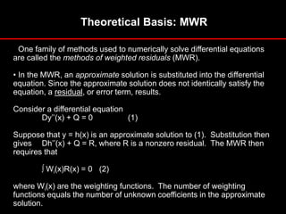
• The variational method involves the integral of a function that
produces a number. Each new function produces a new
number.
• The function that produces the lowest number has the
additional property of satisfying a specific differential equation.
• Consider the integral
p D/2 * y’’(x) - Qy]dx = 0. (1)
The numerical value of pcan be calculated given a specific
equation y = f(x). Variational calculus shows that the
particular equation y = g(x) which yields the lowest numerical
value for pis the solution to the differential equation
Dy’’(x) + Q = 0. (2)

16. Theoretical Basis: Variational Method (cont.)
• In solid mechanics, the so-called Rayeigh-Ritz technique
uses the Theorem of Minimum Potential Energy (with the
potential energy being the functional, p) to develop the
element equations.
• The trial solution that gives the minimum value of pis the
approximate solution.
• In other specialty areas, a variational principle can usually
be found.

17. Sources of Error in the FEM
• The three main sources of error in a typical FEM solution are
discretization errors, formulation errors and numerical errors.
• Discretization error results from transforming the physical
system (continuum) into a finite element model, and can be
related to modeling the boundary shape, the boundary
conditions, etc.
Discretization error due to poor
geometry representation.
Discretization error effectively
eliminated.

18. Sources of Error in the FEM (cont.)
• Formulation error results from the use of elements that don't precisely
describe the behavior of the physical problem.
• Elements which are used to model physical problems for which they are
not suited are sometimes referred to as ill-conditioned or
mathematically unsuitable elements.
• For example a particular finite element might be formulated on the
assumption that displacements vary in a linear manner over the
domain. Such an element will produce no formulation error when it is
used to model a linearly varying physical problem (linear varying
displacement field in this example), but would create a significant
formulation error if it used to represent a quadratic or cubic varying
displacement field.

19. Sources of Error in the FEM (cont.)
• Numerical error occurs as a result of
numerical calculation procedures, and
includes truncation errors and round off
errors.
• Numerical error is therefore a problem mainly
concerning the FEM vendors and developers.
• The user can also contribute to the numerical
accuracy, for example, by specifying a
physical quantity, say Young’s modulus, E, to
an inadequate number of decimal places.

20. Advantages of the Finite Element Method
• Can readily handle complex geometry:
• The heart and power of the FEM.
• Can handle complex analysis types:
• Vibration
• Transients
• Nonlinear
• Heat transfer
• Fluids
• Can handle complex loading:
• Node-based loading (point loads).
• Element-based loading (pressure, thermal, inertial
forces).
• Time or frequency dependent loading.
• Can handle complex restraints:
• Indeterminate structures can be analyzed.

21. Advantages of the Finite Element Method (cont.)
• Can handle bodies comprised of nonhomogeneous materials:
• Every element in the model could be assigned a different
set of material properties.
• Can handle bodies comprised of nonisotropic materials:
• Orthotropic
• Anisotropic
• Special material effects are handled:
• Temperature dependent properties.
• Plasticity
• Creep
• Swelling
• Special geometric effects can be modeled:
• Large displacements.
• Large rotations.
• Contact (gap) condition.

22. Disadvantages of the Finite Element Method
• A specific numerical result is obtained for a specific
problem. A general closed-form solution, which would
permit one to examine system response to changes in
various parameters, is not produced.
• The FEM is applied to an approximation of the mathematical
model of a system (the source of so-called inherited errors.)
• Experience and judgment are needed in order to construct
a good finite element model.
• A powerful computer and reliable FEM software are
essential.
• Input and output data may be large and tedious to prepare
and interpret.

23. Disadvantages of the Finite Element Method (cont.)
• Numerical problems:
• Computers only carry a finite number of significant
digits.
• Round off and error accumulation.
• Can help the situation by not attaching stiff (small)
elements to flexible (large) elements.
• Susceptible to user-introduced modelling errors:
• Poor choice of element types.
• Distorted elements.
• Geometry not adequately modelled.
• Certain effects not automatically included:
• Complex Buckling
• Hybrid composites.
• Nanomaterials modelling .
• Multiple simultaneous causes.

24. Coupled Field Analysis
Module 6

25. • In this, we will briefly describe how to do
a thermal-stress analysis.
• The purpose is two-fold:
– To show you how to apply thermal loads in a
stress analysis.
– To introduce you to a coupled-field analysis.
Coupled Field Analysis
Overview

26. Thermally Induced Stress
• When a structure is heated or cooled,
it deforms by expanding or
contracting.
• If the deformation is somehow
restricted — by displacement
constraints or an opposing pressure,
for example — thermal stresses are
induced in the structure.
• Another cause of thermal stresses is
non-uniform deformation, due to
different materials (i.e, different
coefficients of thermal expansion).
Thermal stresses
due to constraints
Thermal stresses
due to different
materials
Coupled Field Analysis
…Overview

27. • There are two methods of solving thermal-stress problems
using ANSYS. Both methods have their advantages.
– Sequential coupled field
- Older method, uses two element types mapping thermal
results as structural temperature loads
+ Efficient when running many thermal transient time
points but few structural time points
+ Can easily be automated with input files
– Direct coupled field
+ Newer method uses one element type to solve both
physics problems
+ Allows true coupling between thermal and structural
phenomena
- May carry unnecessary overhead for some analyses
Coupled Field Analysis
…Overview

28. • The Sequential method involves two
analyses:
1. First do a steady-state (or transient)
thermal analysis.
• Model with thermal elements.
• Apply thermal loading.
• Solve and review results.
2. Then do a static structural analysis.
• Switch element types to structural.
• Define structural material
properties, including thermal
expansion coefficient.
• Apply structural loading, including
temperatures from thermal
analysis.
• Solve and review results.
Thermal
Analysis
Structural
Analysis
jobname.rth
jobname.rst
Temperatures
Coupled Field Analysis
A. Sequential Method

29. • The Direct Method usually involves just one analysis that
uses a coupled-field element type containing all
necessary degrees of freedom.
1. First prepare the model and mesh
using one of the following coupled
field element types.
• PLANE13 (plane solid).
• SOLID5 (hexahedron).
• SOLID98 (tetrahedron).
2. Apply both the structural and thermal
loads and constraints to the model.
3. Solve and review both thermal and
structural results.
Combined
Thermal
Analysis
Structural
Analysis
jobname.rst
Coupled Field Analysis
B. Direct Method

30. Coupled Field Analysis
Sequential vs. Direct Method
• Direct
– Direct coupling is
advantageous when the
coupled-field interaction is
highly nonlinear and is best
solved in a single solution
using a coupled
formulation.
– Examples of direct coupling
include piezoelectric
analysis, conjugate heat
transfer with fluid flow, and
circuit-electromagnetic
analysis.
• Sequential
– For coupling situations
which do not exhibit a high
degree of nonlinear
interaction, the sequential
method is more efficient
and flexible because you
can perform the two
analyses independently of
each other.
– You can use nodal
temperatures from ANY
load step or time-point in
the thermal analysis as
loads for the stress
analysis. .

31. Case Study 1: Composites in
Microelectronic Packaging
The BOM includes Copper lead frame,
Gold wires for bonding, Silver –epoxy
for die attach, Silicon die and Epoxy
mould composite with Phenolics, Fused
silica powder and Carbon black powder
as the encapsulant materials. Electrical-
Thermal and thermal-structural analyses.

32. Thermal – Structural Results
Displacement Vector sum Von mises stress
Stress intensity XY Shear stress

33. Case Study 2: Composites in
Prosthodontics
Tooth is a functionally graded
composite material with enamel
and dentin. In the third maxillary
molar the occlusal stress can
be 2-3 MPa.
The masticatory heavy chewing
stress will be around 193 MPa.
A composite restorative must with
stand this with an FOS and with
constant hygrothermal attack.

34. Case study 3: Various Buckling
Analyses

35. LINEAR
Eccentric Column

36. Eccentric Column-FEM MODEL

37. x: 0-0.13
y: 0-0.15
x: 0-0.12
y: 0-0.15
FEM METHOD
Load-Deflection Plots

38. FEM MODEL OF HOLLOW
CYLINDER

39. Outer diameter = 158mm
Inner diameter = 138mm
Height = 900mm
Poisson’s ratio = 0.29
Young’s Modulus = 2.15e5 N/mm2
The element used for this model is Solid 186.The
applied pressure is 0.430N/m2. For this analysis
large deformation was set ON and also Arc length
solution was turned ON.
Hollow Cylinder Dimensions

40. FEM METHOD
x: 0-2,y: 0-2.5
TOPOLOGICAL METHOD
x: 0-2, y: 0-2.5
Non-linear
0
0.5
1
1.5
2
2.5
3
0 1 2 3
x
y
x=0.1
1.25y=0.5x (4-x)

41. BI-MODAL BUCKLING
Two coaxial tubes, the inner one
of steel and cross-sectional area
As, and the outer one of
Aluminum alloy and of area Aa,
are compressed between heavy,
flat end plates, as shown in
figure. Assuming that the end
plates are so stiff that both tubes
are shortened by exactly the same
amount.

42. Compression of a Pipe
Pipe-FEM MODEL

43. BI-MODAL BUCKLING
x: 0.2-1
y: 0-0.32
x: 0.2-1
y: 0-0.19
FEM METHOD

44. HINGED SHELL
A hinged cylindrical
shell is subjected to a
vertical point load (P) at
its center.

45. Snap buckling of a hinged shell
Hinged cylindrical shell-FEM MODEL

46. x: 0-1.65
y: 0-1 FEM METHOD
Snap-back buckling of a hinged
shell

47. SNAP-THROUGH BUCKLING
x: 0-1.3
y: 0-1.6
FEM METHOD

48. Case Study 4: Vibration of Composite
Plates
• Vibration studies in composites are
important as the composites are
increasingly being used in automotive,
aerospace and wind energy applications.
• The combined effect of vibrations and
fatigue can degrade a composite further
that is already hygrothermal in affinity.
• The different modes of vibrations are
discussed here.

49. Element selection for ANSYS SOLID 46
3D LAYERED STRUCTURAL SOLID ELEMENT
Element definition
─ Layered version of the 8-node, 3D solid element, solid 45 with three degrees
of freedom per node(UX,UY,UZ).
─ Designed to model thick layered shells or layered solids.
─ can stack several elements to model more than 250 layers to allow through-
the-thickness deformation discontinuities.
Layer definition
─ allows up to 250 uniform thickness layers per element.
─ allows 125 layers with thicknesses that may vary bilinearly.
─ user-input constitutive matrix option.
Options
─ Nonlinear capabilities including large strain.
─Failure criteria through TB,FAIL option.

50. Contd…
Analysis using ANSYS
 After making detailed study of the element library of ANSYS it is
decided that SOLID 46 will be the best suited element for our
problem
 The results obtained from analytical calculation is verified using
a standard analysis package ANSYS

51. SOLID46 3-D 8-Node Layered Structural Solid

52. Finding Storage Modulus (E’)
Using the formula taken from PSG Data Book Page 6.14 Storage
Modulus for the various specimens were determined
Natural frequency F = C√ (gEI/wL4)
where
F – Nodal Frequency
C – Constant
g – Acceleration due to gravity
E – Modulus of elasticity
I – Moment of inertia
L – Effective specimen length
w – Weight of the beam

53. ANSYS MODE SHAPE FOR CARBON FIBRE/EPOXY COMPOSITE
(a) First mode shape (b) second mode shape
(c) Third mode shape (d) Fourth mode shape

54. ANSYS MODE SHAPE FOR GLASS FIBRE/EPOXY COMPOSITE
(a) First mode shape (b) second mode shape
(c) Third mode shape (d) Fourth mode shape

55. ANSYS MODE SHAPE FOR GLASS/POLYPROPYLENE COMPOSITE
(a) First mode shape (b) second mode shape
(c) Third mode shape (d) Fourth mode shape

56. Contd…
TABLE: Frequency of the material analyzed up to 100Hz
Specimen Mode Shape
Natural Frequency (Hz) Storage Modulus E’ (GPa)
ANSYS Experiment ANSYS Experiment
GF-E
I
II
III
IV
1.9301
7.3176
9.7360
13.733
1.855
8.00
9.846
14.22
2.769
1.01
0.23
0.11
2.51
1.21
0.23
0.12
GF-PP
I
II
III
IV
1.913
5.733
9.6281
13.588
1.9104
6.40
9.90
12.799
1.14
0.26
0.11
0.06
1.14
0.32
0.10
0.05
CF-E
I
II
III
IV
1.7270
5.1793
8.7048
12.295
1.73
5.120
8.00
11.81
3.62
0.84
0.30
0.15
3.66
0.82
0.25
0.14

57. Determination of Loss Modulus (E”) and Loss Factor (tan δ)
Following Table shows the values for the loss factor (tan δ) of all specimens considered.
damping results obtained for composite materials studied
Specimen Inertia (m)4 E’ (Gpa) Tan δ E’’ (Gpa) E (Gpa)a
GE 3.25×10-11 12.05 0.0681 0.822 16.19
GPP 1.33×10-10 11.55 0.051 0.586 8.75
CE 1.66×10-11 50.54 0.095 4.806 14.48
a calculated by composite micromechanics approach

58. Case Study 5: Stabilizer Bars for
Four Wheelers
Anti-roll stabilizer bars for four wheelers. Fatigue life
of the stabilizer bars was estimated for qualification.

59. Deflection Plot for Stabilizer Bar

60. Deflection Plot for Stabilizer Tube

61. Equivalent Stresses for Bar

62. Equivalent Stresses for Tube

63. Case Study 6: LCA Generator
• The study deals with modeling, analysis and performance
evaluation of 5kW DC generator assembly. The complete solid
model of the generator with its accessories was modelled using
Pro-Engineer. This paper deals with the structural analysis of
the DC generator casing to find stress and deflection in the
generator casing due to load factor of 9g to which it is
designed. The effect of vibration of generator casing and
hollow shaft with mounting are investigated through detailed
finite element analysis. The bending and torsional natural
frequencies of the hollow shaft are estimated to find the
critical speeds. Torsional frequency of the hollow shaft is
estimated by considering the mass moment of inertias of the
rotating masses. For critical speed analysis of the hollow shaft,
it is considered as simply supported beam with the required
masses and inertias. Then the influence of the critical speeds
due to the casing stiffness is found out analyzing the casing
with the shaft together.

64. Model of LCA Generator

65. Cross-section of the Model

66. Total Deflection at 9g
Maximum deflection of the generator will be 4.761 microns, with-in limits !

67. Von Mises Stresses at 9g
A stress of about 6.756 MPa is much lesser than the Yield Stress of the material

68. Mode Shape of Generator Shaft
Mode shape corresponding to the flexural critical speed (54,972 rpm)
(using solid element TET10 approximation)

69. Conclusions
• The lecture introduced the subject `Introduction to
Finite Element Analysis (FEA) ’ to the undergraduate
audience. The basics, different approaches and the
formulations were outlined in the lecture. Emphasis
was laid on solving structural, mechanical and
multiphysics problems. Understanding the material
behaviour that is a prerequisite to the correct
modelling of the problem was also discussed. Some
engineering applications of the FE approach as
investigated by the speaker were illustrated for the
benefit of the student society and to enable them to
appreciate the depth of the subject field and take it
up as their career .

70. Rig Veda on Infinity
pûrnamadah pûrnamidam pûrnât
pûrnamudacyate pûrnâsya
pûrnamadaya pûrnamevâvasishyate
From infinity is born infinity.
When infinity is taken out of infinity,
only infinity is left over.