
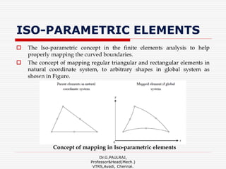
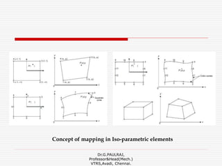
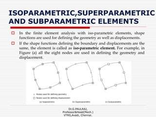
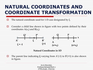
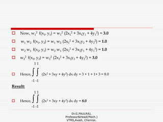
![ or in matrix form
{x} = [N] {x}e
where N are shape functions and (x)e are the coordinates of nodal
points of the element.
The shape functions are to be expressed in natural coordinate system.
For example consider mapping of a rectangular parent element into a
quadrilateral element
Dr.G.PAULRAJ,
Professor&Head(Mech.)
VTRS,Avadi, Chennai.](https://image.slidesharecdn.com/feaunit5-190403041852/85/Finite-Element-Analysis-UNIT-5-7-320.jpg)
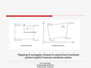
![ The parent rectangular element shown in Figure has nodes 1, 2, 3 and 4
and their coordinates are (–1, –1), (–1, 1), (1, 1) and (1, –1).
The shape functions of this element are
N1 = [(1 − ξ) (1− η)]/4, N2 =[(1+ ξ ) (1− η)]/4
N3 = [(1+ ξ ) (1+ η)]/4 and N4 = [(1- ξ ) (1+ η)]/4
P is a point with coordinate (ξ, η). In global system the coordinates of
the nodal points are (x1, y1), (x2, y2), (x3, y3) and (x4, y4)
Dr.G.PAULRAJ,
Professor&Head(Mech.)
VTRS,Avadi, Chennai.](https://image.slidesharecdn.com/feaunit5-190403041852/85/Finite-Element-Analysis-UNIT-5-9-320.jpg)

![Strain- displacement relationship matrix
J22 -J12 0 0
[B] = 1/ |J| 0 0 -J21 J11 x (1/4)
-J21 J11 J22 -J12
-(1-η) 0 (1- η) 0 (1+ η) 0 -(1+ η) 0
-(1-ε) 0 -(1+ε) 0 (1+ε) 0 (1-ε) 0
x 0 -(1-η) 0 (1- η) 0 (1+ η) 0 -(1+ η)
0 -(1-ε) 0 -(1+ε) 0 (1+ε) 0 (1-ε)
Dr.G.PAULRAJ,
Professor&Head(Mech.)
VTRS,Avadi, Chennai.](https://image.slidesharecdn.com/feaunit5-190403041852/85/Finite-Element-Analysis-UNIT-5-15-320.jpg)
![STIFFNESS MATRIX FOR
4 NODED RECTANGULAR
ELEMENT
Assembling element stiffness matrix for isoparametric element is a
tedious process since it involves co-ordinate transformation form
natural co-ordinate system to global co-ordinate system.
We know that, General element stiffness matrix equation is,
Stiffness matrix, [K] = [B]T [D] [B] dv
v
Dr.G.PAULRAJ,
Professor&Head(Mech.)
VTRS,Avadi, Chennai.
.
P (ξ, η) .
P (x, y)
Parent Element Isoparametric Quadrilateral Element](https://image.slidesharecdn.com/feaunit5-190403041852/85/Finite-Element-Analysis-UNIT-5-16-320.jpg)
![ For Isoparametric quadrilateral element,
[K] =t [B]T [D] [B] ∂x ∂y
For natural co-ordinates,
1 1
[K] =t [B]T [D] [B] x |J| x ∂ε ∂η [∂x ∂y = |J| ∂ε ∂η ]
-1 -1
Where, t = Thickness of the element
|J|= Determinant of the Jacobian
ε , η = Natural coordinates
[B] = Strain- displacement relationship matrix
[D] = Stress-Strain relationship matrix
Dr.G.PAULRAJ,
Professor&Head(Mech.)
VTRS,Avadi, Chennai.](https://image.slidesharecdn.com/feaunit5-190403041852/85/Finite-Element-Analysis-UNIT-5-17-320.jpg)
![ For two dimensional problems,
1 v 0
Stress-Strain relationship matrix, [D] = E/(1-v2) v 1 0
0 0 (1-v)/2
(For plane stress conditions)
1-v v 0
[D] = E/(1+v)(1-2v) v 1-v 0 (For plane strain conditions)
0 0 (1-2v)/2
Where, E = Young’s modulus
v = Poisson’s ratio
Dr.G.PAULRAJ,
Professor&Head(Mech.)
VTRS,Avadi, Chennai.](https://image.slidesharecdn.com/feaunit5-190403041852/85/Finite-Element-Analysis-UNIT-5-18-320.jpg)
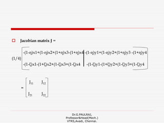
![ P1: Consider a rectangular element as shown in figure. Assume plane
stress condition E= 30x 106 N/m2, v=0.3 and q = [0. 0. 0.002, 0.003, 0.006,
0.0032, 0, 0 ]. Evaluate J, B and D at ξ=0 and η=0.
Solution:
Jacobian matrix J =
-(1-η)x1+(1-η)x2+(1+η)x3-(1+η)x4 -(1-η)y1+(1-η)y2+(1+η)y3 -(1+η)y4
(1/4)
-(1-ξ)x1-(1+ξ)x2+(1-ξ)x3+(1-ξ)x4 -(1-ξ)y1-(1+ξ)y2+(1-ξ)y3+(1-ξ)y4
J J
Dr.G.PAULRAJ,
Professor&Head(Mech.)
VTRS,Avadi, Chennai.
q2
+
C (1, 0.5)
q8
(2, 1)(0, 0)
(2, 1)
(0, 1)
q7
q6
q5
q1
Y
q3
q4
X
3
2
4
1](https://image.slidesharecdn.com/feaunit5-190403041852/85/Finite-Element-Analysis-UNIT-5-19-320.jpg)
![2(1-η)+2(1+η) (1+η) -(1+η) 1 0 J11 J12
J= (1/4) = =
-2(1+ξ)+2(1-ξ) (1+ξ)+(1-ξ) 0 ½ J21 J22
For this rectangular element, we find that J is a constant matrix. Now Strain
displacement relationship matrix
J22 -J12 0 0 -(1-η) 0 (1- η) 0 (1+ η) 0 -(1+ η) 0
[B] =1/|J| 0 0 -J21 J11 x(1/4)x -(1- ξ) 0 -(1+ ξ) 0 (1+ ξ) 0 (1- ξ) 0
-J21 J11 J22 -J12 0 -(1-η) 0 (1- η) 0 (1+ η) 0 -(1+ η)
0 -(1-ε) 0 -(1+ε) 0 (1+ε) 0 (1-ε)
Dr.G.PAULRAJ,
Professor&Head(Mech.)
VTRS,Avadi, Chennai.](https://image.slidesharecdn.com/feaunit5-190403041852/85/Finite-Element-Analysis-UNIT-5-20-320.jpg)
![½ 0 0 0 -¼ 0 ¼ 0 ¼ 0 - ¼ 0
[B] =1/½ 0 0 0 1 x 0 -½ 0 -½ 0 ½ 0 ½
0 0 ½ 0 -½ -¼ -½ ¼ ½ ¼ ½ -¼
The stresses at ξ=0 and η=0
1 v 0
Stress-Strain relationship matrix, [D] = E/(1-v2) v 1 0
(For plane stress conditions) 0 0 (1-v)/2
1 0.3 0
[D] = (30x106)/(1-0.09) 0.03 1 0
0 0 0.35
Dr.G.PAULRAJ,
Professor&Head(Mech.)
VTRS,Avadi, Chennai.](https://image.slidesharecdn.com/feaunit5-190403041852/85/Finite-Element-Analysis-UNIT-5-21-320.jpg)
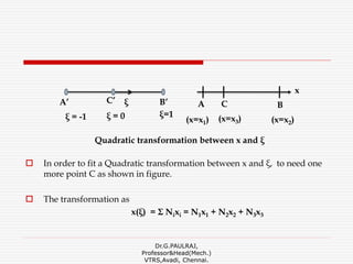
![ An appropriate linear transformation between x and ξ is given by
x(ξ) = [ (x1 + x2)/2 ] + [ (x1 - x2)/2 ] ξ
= [ (1- ξ)/2] x1 + [ (1+ ξ)/2] x2
x(ξ) = N1x1 + N2x2
Where Ni = Interpolation function used for coordinate transformation.
If the shape function used for coordinate transformation are of lower
degree than those for unknown field variable called as Sub-parametric
elements.
If the shape function used for coordinate transformation are of higher
degree than those for unknown field variable called as Superparametric
elements.
Dr.G.PAULRAJ,
Professor&Head(Mech.)
VTRS,Avadi, Chennai.](https://image.slidesharecdn.com/feaunit5-190403041852/85/Finite-Element-Analysis-UNIT-5-28-320.jpg)
![ Rewriting the above equation in the standard notation,
x1
x = [N1 N2]
x2
For point P’, ξ = 0.5, correspondingly,
x = [ (x1 + 3x2)/4 ]
Which is the point P.
For point Q,
x = [ x1 + (x2 + x1)/4 ]
correspondingly, ξ = -0.5,
Which is the point Q’.
Dr.G.PAULRAJ,
Professor&Head(Mech.)
VTRS,Avadi, Chennai.](https://image.slidesharecdn.com/feaunit5-190403041852/85/Finite-Element-Analysis-UNIT-5-29-320.jpg)
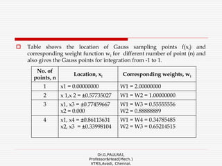


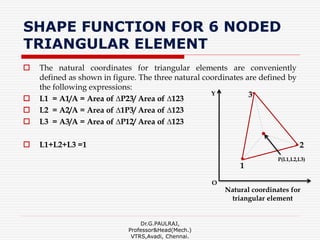
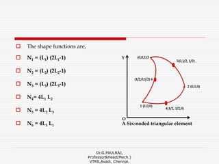
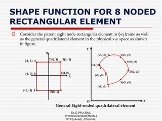
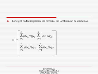
The document discusses isoparametric finite elements. It defines isoparametric, superparametric, and subparametric elements. It provides examples of shape functions for 4-noded rectangular, 6-noded triangular, and 8-noded rectangular isoparametric elements. It also discusses coordinate transformation from the natural to global coordinate system using these shape functions and calculating the Jacobian.