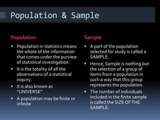
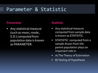
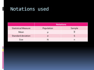
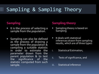
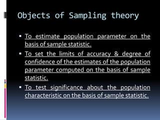
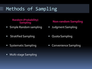
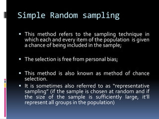
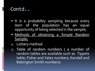
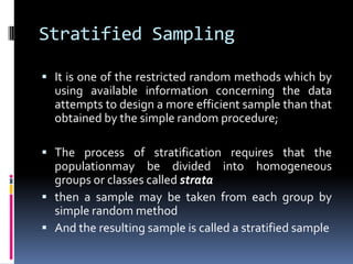
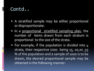
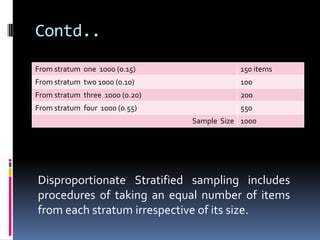
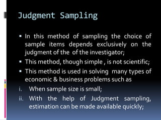
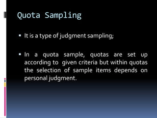
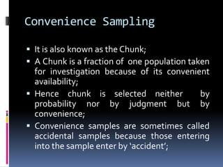
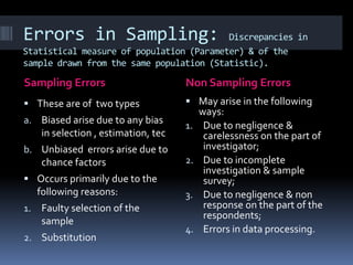
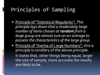
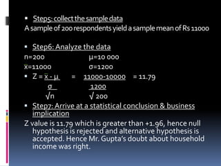
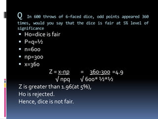
This document provides information on population and sampling concepts. It defines key terms like population, sample, parameter, statistic and discusses different sampling methods like random sampling (simple random sampling, stratified sampling, systematic sampling) and non-random sampling (judgment sampling, quota sampling, convenience sampling).
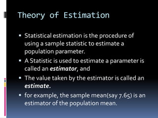
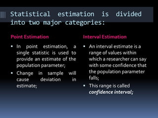
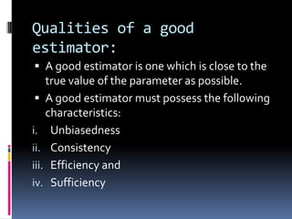
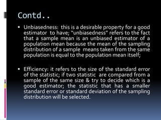
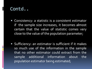
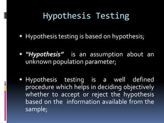
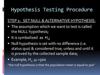
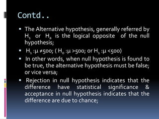
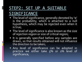
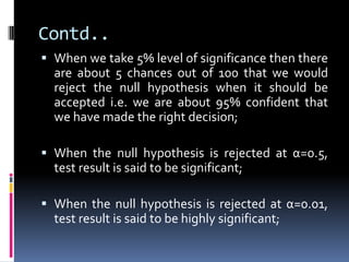
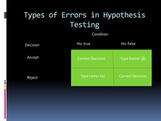
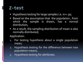
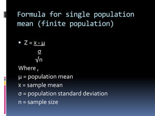
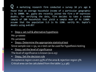
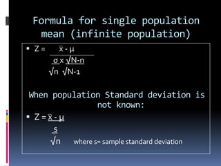
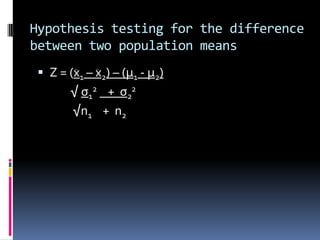
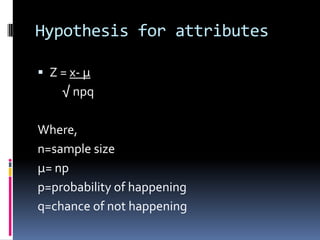
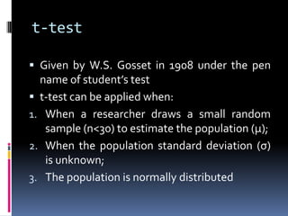
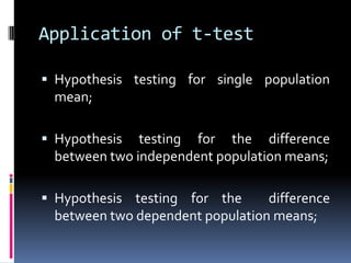
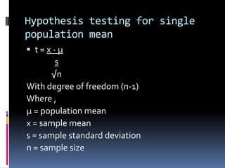
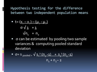
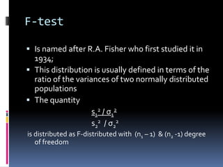
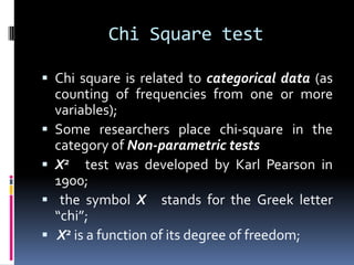
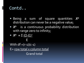
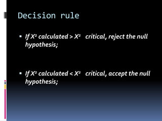
It also discusses the theory of estimation including point estimation and interval estimation. Qualities of a good estimator like unbiasedness, consistency and efficiency are explained. Hypothesis testing procedures including setting null and alternative hypotheses, test statistics, decision rules and types of errors are outlined. Common statistical tests like the z-test and its applications are described.