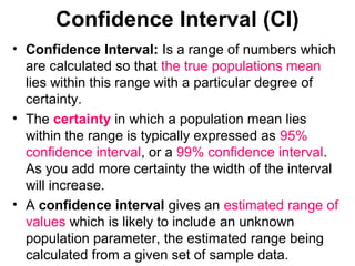
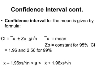
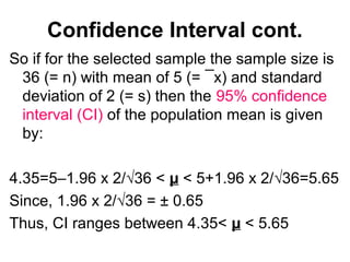
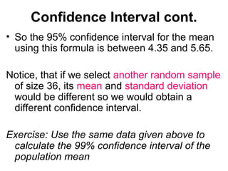
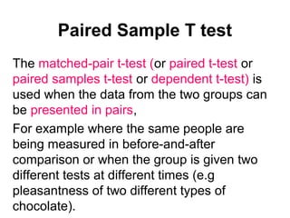
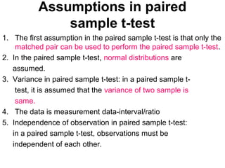
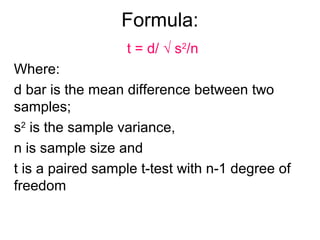
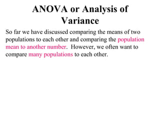
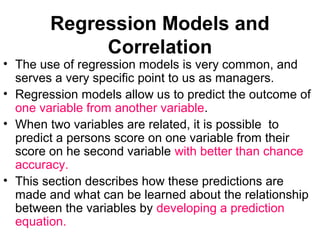
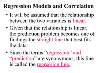
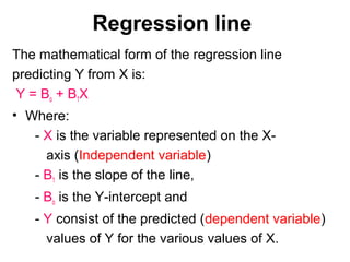
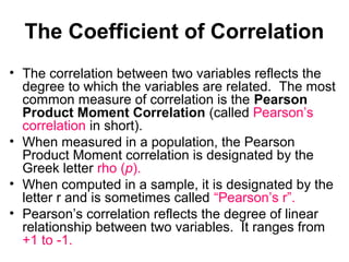
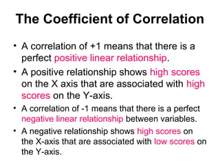
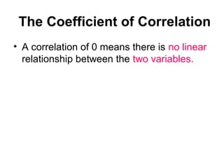
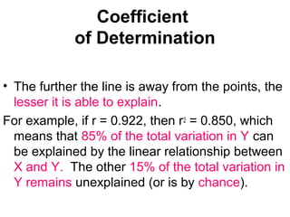
This document provides an overview of key concepts in inferential statistics including parameter estimation, hypothesis testing, t-tests, linear regression, and analysis of variance (ANOVA). It defines important statistical terms like population parameter, point estimate, confidence interval, null and alternative hypotheses, type I and II errors, and significance. Common statistical tests covered include the one sample t-test, independent two sample t-test, and tests assumptions. Linear regression models and correlation are also discussed including the regression line, coefficient of correlation, and coefficient of determination.
The ppt gives an idea about basic concept of Estimation. point and interval. Properties of good estimate is also covered. Confidence interval for single means, difference between two means, proportion and difference of two proportion for different sample sizes are included along with case studies.
Please Subscribe to this Channel for more solutions and lectures
http://www.youtube.com/onlineteaching
Chapter 6: Normal Probability Distribution
6.4: The Central Limit Theorem
Please Subscribe to this Channel for more solutions and lectures
http://www.youtube.com/onlineteaching
Chapter 11: Goodness-of-Fit and Contingency Tables
11.1: Goodness of Fit Notation
Please Subscribe to this Channel for more solutions and lectures
http://www.youtube.com/onlineteaching
Chapter 6: Normal Probability Distribution
6.1: The Standard Normal Distribution
Please Subscribe to this Channel for more solutions and lectures
http://www.youtube.com/onlineteaching
Chapter 10: Correlation and Regression
10.2: Regression
Hypothesis is usually considered as the principal instrument in research and quality control. Its main function is to suggest new experiments and observations. In fact, many experiments are carried out with the deliberate object of testing hypothesis. Decision makers often face situations wherein they are interested in testing hypothesis on the basis of available information and then take decisions on the basis of such testing. In Six –Sigma methodology, hypothesis testing is a tool of substance and used in analysis phase of the six sigma project so that improvement can be done in right direction
Please Subscribe to this Channel for more solutions and lectures
http://www.youtube.com/onlineteaching
Chapter 11: Goodness-of-Fit and Contingency Tables
11.1: Goodness of Fit Notation
Please Subscribe to this Channel for more solutions and lectures
http://www.youtube.com/onlineteaching
Chapter 6: Normal Probability Distribution
6.1: The Standard Normal Distribution
Please Subscribe to this Channel for more solutions and lectures
http://www.youtube.com/onlineteaching
Chapter 10: Correlation and Regression
10.2: Regression
Hypothesis is usually considered as the principal instrument in research and quality control. Its main function is to suggest new experiments and observations. In fact, many experiments are carried out with the deliberate object of testing hypothesis. Decision makers often face situations wherein they are interested in testing hypothesis on the basis of available information and then take decisions on the basis of such testing. In Six –Sigma methodology, hypothesis testing is a tool of substance and used in analysis phase of the six sigma project so that improvement can be done in right direction
Statistical inference: Statistical Power, ANOVA, and Post Hoc testsEugene Yan Ziyou
This deck was used in the IDA facilitation of the John Hopkins' Data Science Specialization course for Statistical Inference. It covers the topics in week 4 (statistical power, ANOVA, and post hoc tests).
The data and R script for the lab session can be found here: https://github.com/eugeneyan/Statistical-Inference
Objectives:
Understand the elements of hypothesis testing for testing a population mean (for large sample):
Identify appropriate null and alternative hypotheses
Select a level of significance
Compute the value of test statistic
Locate a critical or rejection region
Interpret the appropriate conclusion
Inferential Statistics:
It consists of methods for measuring and drawing conclusion about a population based on information obtained from a sample
Estimation (Point & Interval Estimation)
Significance/ Hypothesis Testing
Hypothesis Testing :
Tentative assumption related to certain phenomenon which a researcher want to verify
Allows us to use sample data to test a claim about a population, such as testing whether a population mean equals same number.
Hypothesis:
Hypothesis: An informed guess or a conjecture about a population parameter, which may or may not be true. It tests whether a population parameter is less than, greater than, or equal to a specified value (hypothetical).
A statement of belief used in the evaluation of a population parameter such as the mean of a population.
Example:
Frequent users of narcotics have a mean anger expression score higher than for non-users.
Types of hypotheses:
There are two types of hypotheses.
Null hypothesis (H0):
A claim that there is no difference between the population parameter and the hypothesized value. For example, the mean of a population equals the hypothesized value .
Alternative or Researcher hypothesis (Ha or H1):
A claim that disagrees with the null hypothesis. For example, the mean of a population is not equal to the hypothesized value.
One tailed hypotheses are directional.
Two-tailed hypothesis is otherwise non-directional.
Underlying assumptions for testing of hypothesis for population mean.
The sample has been randomly selected from the population or process.
The underlying population is normally distributed (or if not normally distributed, then n is large say greater than or equal to 30).
Population variance (2) either known or sample variance (s2) assumed to be approximately equal to population variance, when n is large.
Basic Elements of Testing Hypothesis:
Null Hypothesis
Alternative Hypothesis (Researcher Hypothesis)
Choice of appropriate level of significance
Assumptions
Test Statistic (Formula): Application of sample results in the formula to calculate the value of test statistic use for decision purpose.
Rejection Region (Critical Region): Based on alternative hypothesis and level of significance.
Conclusion: If the calculated value of the test statistic falls in the rejection region, reject H0 in favor of Ha, otherwise fail to reject H0.
Steps of Hypothesis Testing:
Step 1: State the hypothesis and identify the claim.
Step 2: State the Level of Significance.
Step 3: Compute the test value (Test Statistics).
Read
Discuss
Courses
Practice
We will be trying to understand the T-Test in R Programming with the help of an example. Suppose a businessman with two sweet shops in a town wants to check if the average number of sweets sold in a day in both stores is the same or not.
So, the businessman takes the average number of sweets sold to 15 random people in the respective shops. He found out that the first shop sold 30 sweets on average whereas the second shop sold 40. So, from the owner’s point of view, the second shop was doing better business than the former. But the thing to notic
Hypothesis Testing Definitions A statistical hypothesi.docxwilcockiris
Hypothesis Testing
Definitions:
A statistical hypothesis is a guess about a population parameter. The guess may or not be
true.
The null hypothesis, written H0, is a statistical hypothesis that states that there is no
difference between a parameter and a specific value, or that there is no difference between
two parameters.
The alternative hypothesis, written H1 or HA, is a statistical hypothesis that specifies a
specific difference between a parameter and a specific value, or that there is a difference
between two parameters.
Example 1:
A medical researcher is interested in finding out whether a new medication will have
undesirable side effects. She is particularly concerned with the pulse rate of patients who
take the medication. The research question is, will the pulse rate increase, decrease, or
remain the same after a patient takes the medication?
Since the researcher knows that the mean pulse rate for the population under study is 82
beats per minute, the hypotheses for this study are:
H0: µ = 82
HA: µ ≠ 82
The null hypothesis specifies that the mean will remain unchanged and the alternative
hypothesis states that it will be different. This test is called a two-tailed test since the
possible side effects could be to raise or lower the pulse rate. Notice that this is a non
directional hypothesis. The rejection region lies in both tails. We divide the alpha in two
and place half in each tail.
Example 2:
An entrepreneur invents an additive to increase the life of an automobile battery. If the
mean lifetime of the automobile battery is 36 months, then his hypotheses are:
H0: µ ≤ 36
HA: µ > 36
Here, the entrepreneur is only interested in increasing the lifetime of the batteries, so his
alternative hypothesis is that the mean is greater than 36 months. The null hypothesis is
that the mean is less than or equal to 36 months. This test is one-tailed since the interest
is only in an increased lifetime. Notice that the direction of the inequality in the alternate
hypothesis points to the right, same as the area of the curve that forms the rejection
region.
Example 3:
A landlord who wants to lower heating bills in a large apartment complex is considering
using a new type of insulation. If the current average of the monthly heating bills is $78,
his hypotheses about heating costs with the new insulation are:
H0: µ ≥ 78
HA: µ < 78
This test is also a one-tailed test since the landlord is interested only in lowering heating
costs. Notice that the direction of the inequality in the alternate hypothesis points to the
left, same as the area of the curve that forms the rejection region.
Study Design:
After stating the hypotheses, the researcher’s next step is to design the study. In designing
the study, the researcher selects an appropriate statistical test, chooses a level of
significance, and formulates a plan for conducting the study..
tests of significance in periodontics aspect, tests of significance with common examples, tests in brief, null hypothesis, parametric vs non parametric tests, seminar by sai lakshmi
Embracing GenAI - A Strategic ImperativePeter Windle
Artificial Intelligence (AI) technologies such as Generative AI, Image Generators and Large Language Models have had a dramatic impact on teaching, learning and assessment over the past 18 months. The most immediate threat AI posed was to Academic Integrity with Higher Education Institutes (HEIs) focusing their efforts on combating the use of GenAI in assessment. Guidelines were developed for staff and students, policies put in place too. Innovative educators have forged paths in the use of Generative AI for teaching, learning and assessments leading to pockets of transformation springing up across HEIs, often with little or no top-down guidance, support or direction.
This Gasta posits a strategic approach to integrating AI into HEIs to prepare staff, students and the curriculum for an evolving world and workplace. We will highlight the advantages of working with these technologies beyond the realm of teaching, learning and assessment by considering prompt engineering skills, industry impact, curriculum changes, and the need for staff upskilling. In contrast, not engaging strategically with Generative AI poses risks, including falling behind peers, missed opportunities and failing to ensure our graduates remain employable. The rapid evolution of AI technologies necessitates a proactive and strategic approach if we are to remain relevant.
The French Revolution, which began in 1789, was a period of radical social and political upheaval in France. It marked the decline of absolute monarchies, the rise of secular and democratic republics, and the eventual rise of Napoleon Bonaparte. This revolutionary period is crucial in understanding the transition from feudalism to modernity in Europe.
For more information, visit-www.vavaclasses.com
Biological screening of herbal drugs: Introduction and Need for
Phyto-Pharmacological Screening, New Strategies for evaluating
Natural Products, In vitro evaluation techniques for Antioxidants, Antimicrobial and Anticancer drugs. In vivo evaluation techniques
for Anti-inflammatory, Antiulcer, Anticancer, Wound healing, Antidiabetic, Hepatoprotective, Cardio protective, Diuretics and
Antifertility, Toxicity studies as per OECD guidelines
Unit 8 - Information and Communication Technology (Paper I).pdfThiyagu K
This slides describes the basic concepts of ICT, basics of Email, Emerging Technology and Digital Initiatives in Education. This presentations aligns with the UGC Paper I syllabus.
Acetabularia Information For Class 9 .docxvaibhavrinwa19
Acetabularia acetabulum is a single-celled green alga that in its vegetative state is morphologically differentiated into a basal rhizoid and an axially elongated stalk, which bears whorls of branching hairs. The single diploid nucleus resides in the rhizoid.
June 3, 2024 Anti-Semitism Letter Sent to MIT President Kornbluth and MIT Cor...Levi Shapiro
Letter from the Congress of the United States regarding Anti-Semitism sent June 3rd to MIT President Sally Kornbluth, MIT Corp Chair, Mark Gorenberg
Dear Dr. Kornbluth and Mr. Gorenberg,
The US House of Representatives is deeply concerned by ongoing and pervasive acts of antisemitic
harassment and intimidation at the Massachusetts Institute of Technology (MIT). Failing to act decisively to ensure a safe learning environment for all students would be a grave dereliction of your responsibilities as President of MIT and Chair of the MIT Corporation.
This Congress will not stand idly by and allow an environment hostile to Jewish students to persist. The House believes that your institution is in violation of Title VI of the Civil Rights Act, and the inability or
unwillingness to rectify this violation through action requires accountability.
Postsecondary education is a unique opportunity for students to learn and have their ideas and beliefs challenged. However, universities receiving hundreds of millions of federal funds annually have denied
students that opportunity and have been hijacked to become venues for the promotion of terrorism, antisemitic harassment and intimidation, unlawful encampments, and in some cases, assaults and riots.
The House of Representatives will not countenance the use of federal funds to indoctrinate students into hateful, antisemitic, anti-American supporters of terrorism. Investigations into campus antisemitism by the Committee on Education and the Workforce and the Committee on Ways and Means have been expanded into a Congress-wide probe across all relevant jurisdictions to address this national crisis. The undersigned Committees will conduct oversight into the use of federal funds at MIT and its learning environment under authorities granted to each Committee.
• The Committee on Education and the Workforce has been investigating your institution since December 7, 2023. The Committee has broad jurisdiction over postsecondary education, including its compliance with Title VI of the Civil Rights Act, campus safety concerns over disruptions to the learning environment, and the awarding of federal student aid under the Higher Education Act.
• The Committee on Oversight and Accountability is investigating the sources of funding and other support flowing to groups espousing pro-Hamas propaganda and engaged in antisemitic harassment and intimidation of students. The Committee on Oversight and Accountability is the principal oversight committee of the US House of Representatives and has broad authority to investigate “any matter” at “any time” under House Rule X.
• The Committee on Ways and Means has been investigating several universities since November 15, 2023, when the Committee held a hearing entitled From Ivory Towers to Dark Corners: Investigating the Nexus Between Antisemitism, Tax-Exempt Universities, and Terror Financing. The Committee followed the hearing with letters to those institutions on January 10, 202
2024.06.01 Introducing a competency framework for languag learning materials ...Sandy Millin
http://sandymillin.wordpress.com/iateflwebinar2024
Published classroom materials form the basis of syllabuses, drive teacher professional development, and have a potentially huge influence on learners, teachers and education systems. All teachers also create their own materials, whether a few sentences on a blackboard, a highly-structured fully-realised online course, or anything in between. Despite this, the knowledge and skills needed to create effective language learning materials are rarely part of teacher training, and are mostly learnt by trial and error.
Knowledge and skills frameworks, generally called competency frameworks, for ELT teachers, trainers and managers have existed for a few years now. However, until I created one for my MA dissertation, there wasn’t one drawing together what we need to know and do to be able to effectively produce language learning materials.
This webinar will introduce you to my framework, highlighting the key competencies I identified from my research. It will also show how anybody involved in language teaching (any language, not just English!), teacher training, managing schools or developing language learning materials can benefit from using the framework.
Macroeconomics- Movie Location
This will be used as part of your Personal Professional Portfolio once graded.
Objective:
Prepare a presentation or a paper using research, basic comparative analysis, data organization and application of economic information. You will make an informed assessment of an economic climate outside of the United States to accomplish an entertainment industry objective.
Honest Reviews of Tim Han LMA Course Program.pptxtimhan337
Personal development courses are widely available today, with each one promising life-changing outcomes. Tim Han’s Life Mastery Achievers (LMA) Course has drawn a lot of interest. In addition to offering my frank assessment of Success Insider’s LMA Course, this piece examines the course’s effects via a variety of Tim Han LMA course reviews and Success Insider comments.
2. Overview
In this lesson, we will briefly cover a few main concepts
used in inferential Statistics, such as estimating a
population parameter, hypothesis testing, T-tests, linear
regression and Analysis of Variance (ANOVA).
After completing this section you should be able to do
the following:
Recognize common inferential statistical tests
Identify and compute basic point estimates of population
parameters
Describe the basics of hypothesis testing
Understand and identify the use of regression modeling
3. Introduction
• Inferential Statistics’ are mathematical
tools that permits the researcher to
generalize to a population of individuals
based upon information obtained from a
limited number of research participants
(the sample).
4. Example
• For instance, consider an experiment where sales
were increased by 25% following a media
advertisement on 10 products compared to sales of 10
products which were not advertised. Inferential
Statistics allows us to decide if the increased sales are
due to chance or from the effect of advertising.
• There are primarily two ways to use inferential
statistics:
• Parameter Estimation
• Test of Hypothesis
5. Parameter Estimation
• A Parameter is any of the factors that
limits the way in which something can
be done.
• Parameter estimation falls into two
Categories:
• Point estimation
• Confidence interval (CI) estimation
6. Point Estimation
• Point estimation: The Estimate or Prediction
of a population parameter is often referred to as
a Point estimate.
• That is to say, the estimate is a single value
based on a sample, a statistic, which is then
used to estimate the corresponding value in the
population (a parameter).
• The average (mean = a parameter) of our
sample can be used as an estimator of the
population mean.
7. Sampling Error
• Sampling Error: the difference between the
population value of interest (e.g. mean), and
the sample value. Our sample value is often
referred to as an estimate of our population
value.
• If the sample is randomly drawn from the
population, then sampling error will be random
and will be distributed normally.
8. Confidence Interval (CI)
• Confidence Interval: Is a range of numbers which
are calculated so that the true populations mean
lies within this range with a particular degree of
certainty.
• The certainty in which a population mean lies
within the range is typically expressed as 95%
confidence interval, or a 99% confidence interval.
As you add more certainty the width of the interval
will increase.
• A confidence interval gives an estimated range of
values which is likely to include an unknown
population parameter, the estimated range being
calculated from a given set of sample data.
9. Confidence Interval cont.
• Confidence interval for the mean is given by
formula:
CI = ¯x ± Zα s/√n ¯x = mean
Zα = constant for 95% CI
= 1.96 and 2.56 for 99%
¯x – 1.96xs/√n < µ < ¯x + 1.96xs/√n
10. Confidence Interval cont.
So if for the selected sample the sample size is
36 (= n) with mean of 5 (= ¯x) and standard
deviation of 2 (= s) then the 95% confidence
interval (CI) of the population mean is given
by:
4.35=5–1.96 x 2/√36 < µ < 5+1.96 x 2/√36=5.65
Since, 1.96 x 2/√36 = ± 0.65
Thus, CI ranges between 4.35< µ < 5.65
11. Confidence Interval cont.
• So the 95% confidence interval for the mean
using this formula is between 4.35 and 5.65.
Notice, that if we select another random sample
of size 36, its mean and standard deviation
would be different so we would obtain a
different confidence interval.
Exercise: Use the same data given above to
calculate the 99% confidence interval of the
population mean
12. Confidence Interval cont.
• If independent samples are taken repeatedly
from the same population, and a confidence
interval calculated for each sample, then a
certain percentage (confidence level) of the
intervals will include the unknown population
parameter.
• Confidence intervals are usually calculated
so that this percentage is 95%, but we can
produce 90%, 99%, 99.9% (or whatever)
confidence intervals for the unknown
parameter.
13. Confidence Interval cont.
• The width of the confidence interval gives us
some idea about how uncertain we are about
unknown parameter.
• A very wide interval may indicate that more
data should be collected before anything very
definite can be said about the parameter.
• Confidence intervals are more informative than
the simple results of hypothesis tests (where
we decide “reject Ho” or “don’t reject Ho”) since
they provide a range of plausible values for the
unknown parameter.
14. Confidence Interval cont.
• Confidence limits are the lower and the upper
boundaries/values of a confidence interval, that
is, the values which define the range of a
confidence interval.
• The upper and lower bounds of a 95%
confidence interval are the 95% confidence
limits. Such limits may be taken for other
confidence levels, for example, 90%, 99%,
99.9%.
15. Hypothesis Testing
• The second type of inferential statistics is
hypothesis testing. This is sometimes called
statistical testing as well.
• In point estimation and in constructing
confidence interval, we had no expectations
about the values we calculated, whereas in
hypothesis testing we have formed some
expectation about the population parameter.
16. HYPOTHESIS TESTING cont.
Example
• Our hypothesis is that “tree mortality after a particular
forest fire will be greater than 60%”, in other words average
tree mortality > 60%.
• Once our notion of the population parameter has been
developed, we can write two contradictory hypotheses:
The first is research (or alternative) hypothesis, which in
our case is that “the mean tree mortality > 60%”.
The second hypothesis is called the null hypothesis, and is
the opposite of our research hypothesis. In our example, the
null hypothesis would be stated as “the mean tree mortality is
less than or equal to 60%”.
17. Hypothesis Testing cont.
Basic Concepts in Test of Hypothesis
• Def.: A Hypothesis is a tentative explanation
for an observation, phenomenon, or scientific
problem that can be tested by further
investigation.
18. Null and Alternative Hypothesis
• Null Hypothesis: The null hypothesis, (Ho),
represents a theory that has been put forward, either
because it is believed to be true or because it is to be
used as a basis for argument, but has not been
proved.
• For example, in a clinical trial of a new drug, the null
hypothesis might be that “the new drug is no better,
on average, than the current drug”.
We would write
Ho: there is no difference between the two drugs on
average.
19. Null and Alternative Hypothesis
• Alternative Hypothesis: The alternative
hypothesis, H1, is a statement of what a
statistical hypothesis test is set to establish.
• For example, in a clinical trial of a new drug,
the alternative hypothesis might be that “the
new drug has a different effect, on average,
compared to that of the current drug,
We would write:
• H1: the two drugs have different effects, on
average.
20. Null and Alternative Hypothesis
• The alternative hypothesis might also be
that the new drug is better, on average,
than the current drug.
In this case we would write:
• H1: the new drug is better than the current
drug, on average.
21. Null and Alternative Hypothesis
• We give special consideration to the null hypothesis. This
is due to the fact that the null hypothesis relates to the
statement of being tested, whereas the alternative
hypothesis relates to the statement to be accepted if /when
the null is rejected.
• The final conclusion once the test has been carried out is
always given in terms of the null hypothesis. We either
reject Ho in favor of H1 or do not reject Ho.
We never conclude, Reject H1 or even Accept H1.
• We conclude “Do not reject Ho”, this does not necessarily
mean that the null hypothesis is true, it only suggests that
there is not sufficient evidence against Ho in favor of H1.
Rejecting the null hypothesis then, suggests that the
alternative hypothesis may be true.
22. One and Two Tailed Tests
One Tailed Tests (T-Test)
Example
• Our hypothesis is that tree mortality after a
particular forest fire will be greater that 60%.
In other words average tree mortality > 60%.
• In this example, it is a one-tailed test.
Here we were simply considering the idea
that the population mean was larger than
some number. So we would reject the null
hypothesis if we had large values of tree
mortality.
23. Two Tailed Tests cont.
A two-tailed test is used when a research hypothesis is
stated as the following:
Example
• “Tree mortality following fire will be equal to 60%”,
whereas
• our null hypothesis would read “tree mortality
following fire is not equal to 60%”.
• Under this scenario, we could reject our research
hypothesis if tree mortality was much larger than 60
or much smaller than 60.
• This is a two-tailed test
24. Significance
Significance
• The probability of an outcome given the
null hypothesis is a p-value.
• A low probability value indicates rejection
of the null hypothesis.
• Typically: reject Ho if p-value ≤ 0.05 (for a
95% levels of significance test) or 0.01 (for
a 99% levels of significance test).
Statistically, significant means the effect is
not due to chance.
25. Type I and II Errors
Type I and II Errors
• We define a type I error as the event of rejecting
the null hypothesis when the null hypothesis was
true. The probability of a type I error (a) is called
the significance level.
• We define type II error (with probability b) as the
event of failing to reject the null hypothesis when
the null hypothesis was false.
• The type I risk is the chance of deciding that a
significant effect is present when it isn’t.
• The type II risk is the chance of not detecting a
significance effect when one exists.
26. Test of Hypothesis
Steps in Test of Hypothesis
The usual process of hypothesis testing
consists of four steps:
• Formulate the null hypothesis Ho
(commonly, that the observations are the
result of pure chance)
• and the alternative hypothesis H1
(commonly, that the observations show a
real effect combined with a component of
chance variation).
• Identify a test statistic that can be used to
assess the truth of the null hypothesis.
27. Test of Hypothesis cont.
• Compute the P-value, which is the probability
that a test statistic at least as significant as
the one observed would be obtained
assuming that the null hypothesis were true.
The smaller the P-value, the stronger the
evidence against the null hypothesis.
• Compare the P-value to an acceptable
significance value α (sometimes called an
alpha value). If P≤ α, that the observed
effect is statistically significant, the null
hypothesis is ruled out, and the alternative
hypothesis is valid.
29. Regression Models and
Correlation
• The use of regression models is very common, and
serves a very specific point to us as managers.
• Regression models allow us to predict the outcome of
one variable from another variable.
• When two variables are related, it is possible to
predict a persons score on one variable from their
score on he second variable with better than chance
accuracy.
• This section describes how these predictions are
made and what can be learned about the relationship
between the variables by developing a prediction
equation.
30. Regression Models and Correlation
• It will be assumed that the relationship
between the two variables is linear.
• Given that the relationship is linear,
the prediction problem becomes one of
findings the straight line that best fits
the data.
• Since the terms “regression” and
“prediction” are synonymous, this line
is called the regression line.
31. Regression line
The mathematical form of the regression line
predicting Y from X is:
Y = Bo + B1X
• Where:
- X is the variable represented on the X-
axis (Independent variable)
- B1 is the slope of the line,
- Bo is the Y-intercept and
- Y consist of the predicted (dependent variable)
values of Y for the various values of X.
32. The Coefficient of Correlation
• The correlation between two variables reflects the
degree to which the variables are related. The most
common measure of correlation is the Pearson
Product Moment Correlation (called Pearson’s
correlation in short).
• When measured in a population, the Pearson
Product Moment correlation is designated by the
Greek letter rho (p).
• When computed in a sample, it is designated by the
letter r and is sometimes called “Pearson’s r”.
• Pearson’s correlation reflects the degree of linear
relationship between two variables. It ranges from
+1 to -1.
33. The Coefficient of Correlation
• A correlation of +1 means that there is a
perfect positive linear relationship.
• A positive relationship shows high scores
on the X axis that are associated with high
scores on the Y-axis.
• A correlation of -1 means that there is a perfect
negative linear relationship between variables.
• A negative relationship shows high scores on
the X-axis that are associated with low scores on
the Y-axis.
34. The Coefficient of Correlation
• A correlation of 0 means there is no linear
relationship between the two variables.
35. Coefficient
of Determination
• The coefficient of determination r2 gives the proportion
of the variance (fluctuation) of one variable that is
predictable from the other variables.
• It is a measure that allows us to determine how certain
one can be in making predictions from a certain
model/graph.
• The coefficient of determination is a measure of how
well the regression line represents the data.
• If the regression line passes exactly through every
point on the scatter plot, it would be able to explain all
of the variation.
36. Coefficient
of Determination
• The further the line is away from the points, the
lesser it is able to explain.
For example, if r = 0.922, then r2 = 0.850, which
means that 85% of the total variation in Y can
be explained by the linear relationship between
X and Y. The other 15% of the total variation in
Y remains unexplained (or is by chance).
37. T-test
• The T-test gives an indication of the separateness of two sets
of measurements, and is thus used to check whether two sets
of measures are essentially different.
• In many situations, we will want to compare two populations
parameters. To compare these two populations, we can
compare the differences between the two sample means.
• T-test looks for significant difference in means between two
samples or between a population and a sample.
There are 3 types of T-tests;
- One sample T-test
- Independent 2 samples T-test
- Paired sample T-test
38. One Sample T-test
• One sample t-test: is a statistical procedure that is
used to know the mean differences between the
sample and the known value of the population
mean.
• In one sample t-test, we know the population mean.
We draw a random sample from the population and
then compare the sample mean with the population
mean and make a statistical decision as to whether
or not the sample mean is different from the
population.
39. Assumptions in One Sample
t-test
• In one sample t-test, dependent variables should be
normally distributed.
• In one sample t-test, samples drawn from the
population should be random.
• In one sample t-test, cases of the samples should be
independent
• The data is measurement data-interval/ratio
• In one sample t-test, we should know the
population mean.
40. Formula
t = (X1 – µ)/sx
Where: X1= Sample mean
µ = Population mean
Sx = Standard error of the mean
41. Independent t-test
Independent t-test: the independent-
measures t-test (or independent t-test) is
used when measures from the two samples
being compared do not come in matched
pairs. It is used when groups are
independent.
42. Related Formula
t = x1 – x2/√{s2 (1/n1 + 1/n2)}
For an independent 2 sample t-test, it is
important to know if the 2 samples have
similar variances as we interpret data. The
requirement for variance homogeneity test
may be measure with Levine’s test. Results
for this can be given in SPSS along with the t-
test results.
43. Assumption in 2 sample
independence T-test
1.0 Normality: Assumes that the population distributions are
normal. The t-test is quite robust over moderate violations
of this assumption. It is especially robust if a two tailed test
is used and if the sample sizes are not especially small.
Check for normality by creating a histogram.
2.0 Independent Observations: The
observations within each treatment condition
must be independent.
44. Assumption in 2 sample independence
t-test cont.
3.0 Equal Variances: Assume that the
population distributions have the same
variance. This assumption is quite important
(If it is violated, it makes the test’s averaging
of the 2 variances meaningless).
If it is violated, then use a modification of the t-
test procedures as needed. See
“Understanding the Output” in this section for
how to check this with Levenes Test for Equality
of Variances.
45. Paired Sample T test
The matched-pair t-test (or paired t-test or
paired samples t-test or dependent t-test) is
used when the data from the two groups can
be presented in pairs,
For example where the same people are
being measured in before-and-after
comparison or when the group is given two
different tests at different times (e.g
pleasantness of two different types of
chocolate).
46. Assumptions in paired
sample t-test
1. The first assumption in the paired sample t-test is that only the
matched pair can be used to perform the paired sample t-test.
2. In the paired sample t-test, normal distributions are
assumed.
3. Variance in paired sample t-test: in a paired sample t-
test, it is assumed that the variance of two sample is
same.
4. The data is measurement data-interval/ratio
5. Independence of observation in paired sample t-test:
in a paired sample t-test, observations must be
independent of each other.
47. Formula:
t = d/ √ s2
/n
Where:
d bar is the mean difference between two
samples;
s2
is the sample variance,
n is sample size and
t is a paired sample t-test with n-1 degree of
freedom
48. ANOVA or Analysis of
Variance
So far we have discussed comparing the means of two
populations to each other and comparing the population
mean to another number. However, we often want to
compare many populations to each other.
49. ANOVA or Analysis of Variance
Example:
We may want to compare regeneration rates for three
different tree species in northern Idaho. We would begin by
taking samples from each population and then calculate the
means from the three samples and make an inference about
the population means from this.
It is common since these three mean regeneration rates
would all be different numbers however, this does not mean
that there is a difference between the population means for
the three tree types.
To answer that question we can use a statistical test called
an analysis of variance or ANOVA. This test is widely used in
natural resources, and you are bound to come across it when
reading scientific literature.
50. The ANOVA Assumptions
The use of an ANOVA assumes that:
• All the populations are normally distributed (follow a bell
shaped curve)
• All the population variances are equal,
• And all the samples were taken independently of each other
and are randomly collected from their population.
Generally, our null hypothesis when conducting an ANOVA is
that all the population means are equal and our research
(alternative) hypothesis will be that at least one of the
population means is not equal.
51. The ANOVA Assumptions
Although an ANOVA is widely used and it does
indicate that a population mean is different
than others, it does not tell us which one is
different from the others.
Analysis of variance tests the null hypothesis
that all the population means are equal:
Formula:
Ho: µ1 = µ2 = µ3……. = µa
You can read more from Text books
52. The ANOVA cont.
• By comparing two estimates of variance (………) recall that ……….. is the
variance within each of the “a” treatment populations.) one estimate (called
the mean square error or MSE for short) is based on the variances within
the samples. The MSE is an estimate of ………. Whether or not the null
hypothesis is true. The second estimate (mean square between or MSB for
short) is based on the variance of the sample means. The MSB is only an
estimate of ………. If the null hypothesis is true. If the null hypothesis is
false then MSB estimates something larger than ……… The logic by which
analysis of variance tests the null hypothesis is as follows: if the null
hypothesis is true, then MSE and MSB should be about the same since they
are both estimates of the same quantity (…): however, if the null hypothesis
is false then MSB can be expected to be larger than MSE since MSB is
estimating a quantity larger than ……..
• Therefore, if MSB is sufficiently larger than MSE, the null hypothesis can be
rejected. If MSB is not sufficiently larger than MSE then the null hypothesis
cannot be rejected. How much larger is sufficiently larger.
53. END
•Questions
•Next Class
•Assignments
•AOB
Prof. Joseph M. Keriko
Principal, JKUAT - Nairobi Campus
Professor of Organic Chemistry and
EIA/EA Leader Expert
P.O. Box 39125 – 00623 Nairobi
Tel. 0722-915026
Email: kerikojm@yahoo.co.uk