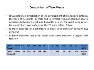
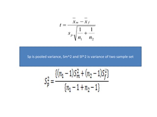
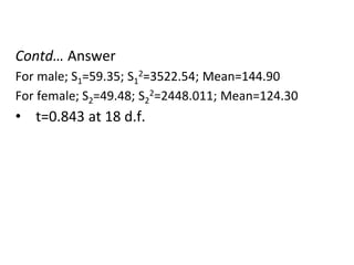
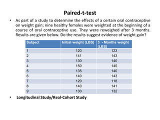
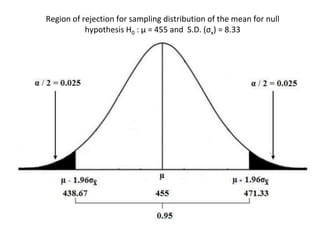
The document discusses statistical inference and hypothesis testing, explaining descriptive and inferential statistics. It outlines key concepts such as population, sample, parameters, and hypotheses, as well as the procedures for hypothesis testing including steps, types of errors, level of significance, and confidence intervals. Additionally, it covers the properties of normal distribution and the implications of using Student's t-distribution for small sample sizes.

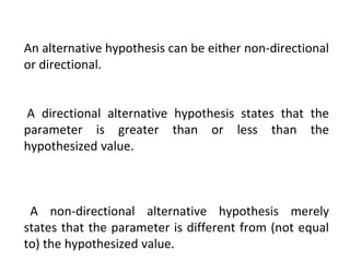
![Type-I and Type-II Errors in Decision Making
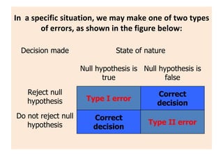
In a specific situation, we may make one of two types of
errors, as shown in the figure below:
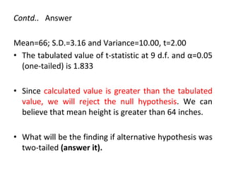
Decision taken by
the investigator
Existing Reality
Group A=Group B Group A # Group B
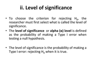
Group A # Group B P[ Type-I Error]
(Level of significance)
Correct Decision
(Power of the study)
Group A=Group B Correct Decision
(Level of confidence)
Type – II Error](https://image.slidesharecdn.com/lecturehypothesistesting-240716163036-03274f4a/85/Lecture_Hypothesis_Testing-statistics-pptx-37-320.jpg)