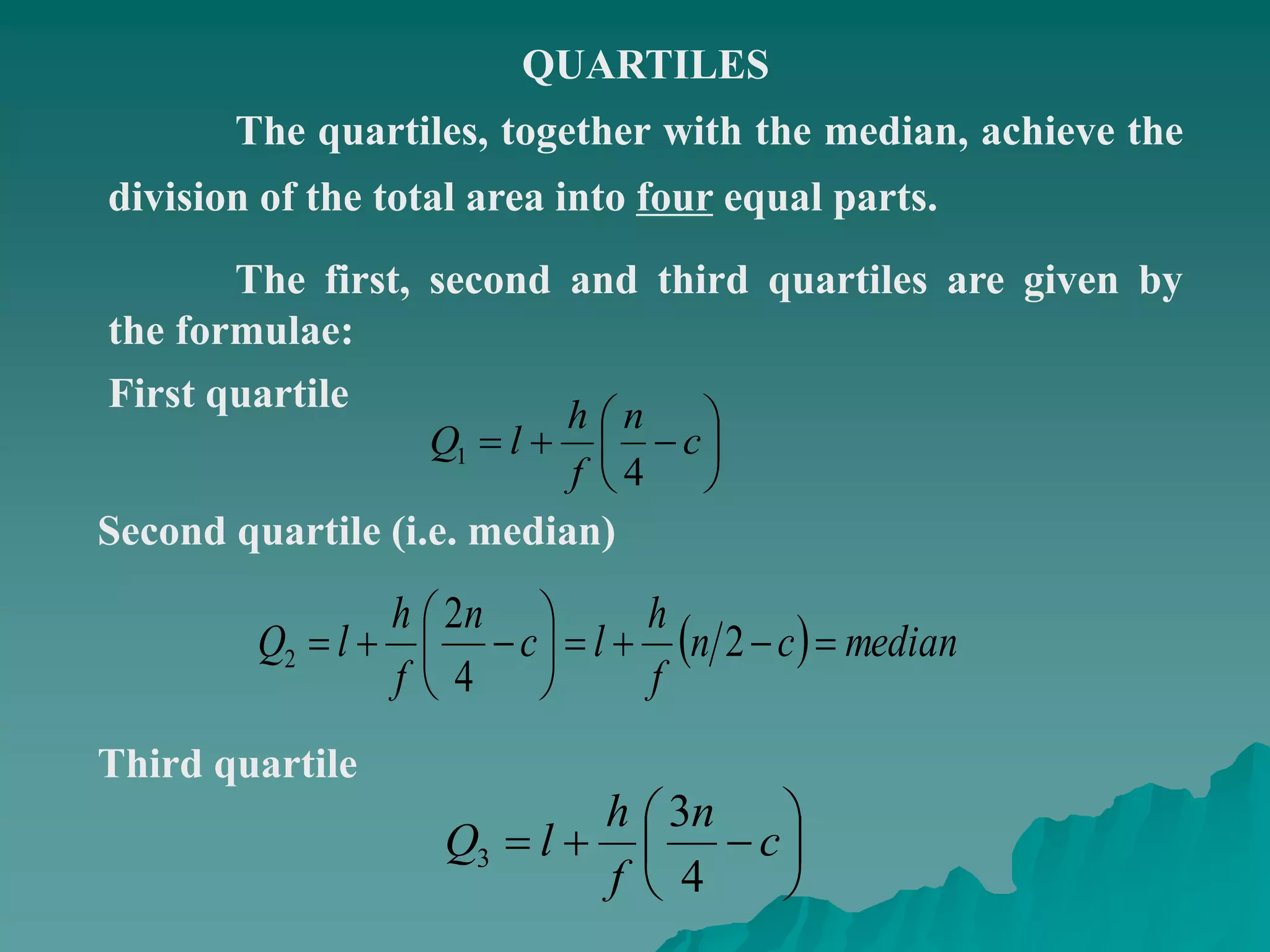
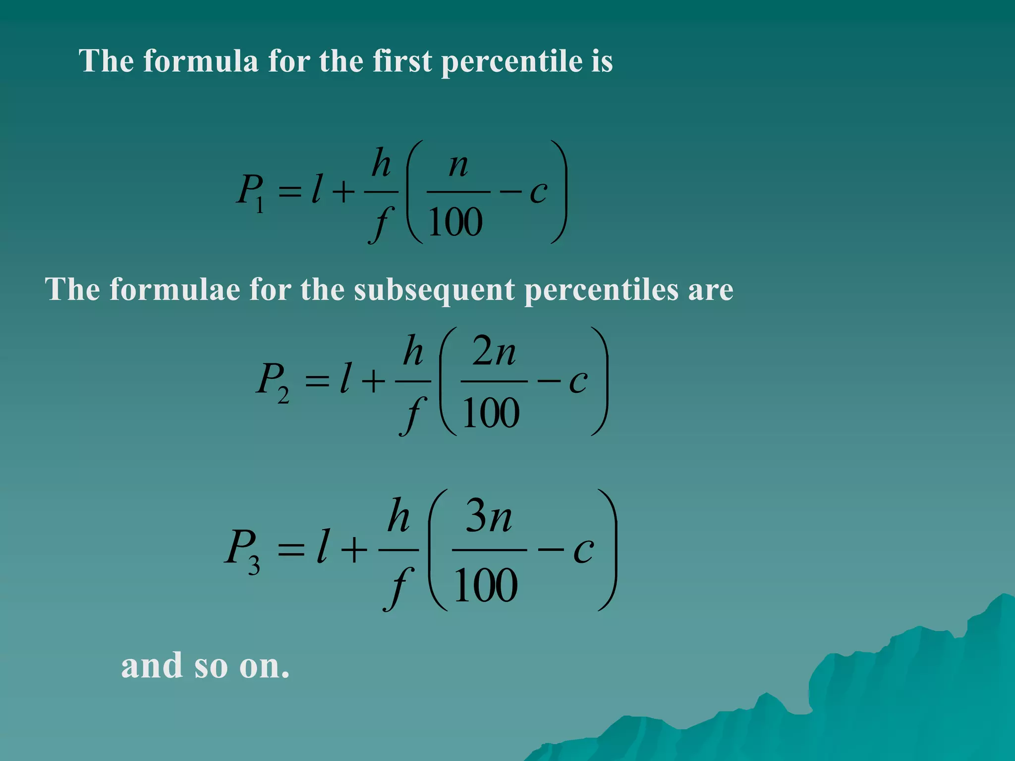
Quartiles, Deciles and Percentiles

1. Quartiles, Deciles and Percentiles
 Let us now extend the concept of
partitioning of the frequency
distribution by taking up the concept
of quantiles (i.e. quartiles, deciles and
percentiles)
 We have already seen that the
median divides the area under the
frequency polygon into two equal
halves:

2. 50% 50%
X
f
Median
A further split to produce quarters, tenths or
hundredths of the total area under the frequency polygon
is equally possible, and may be extremely useful for
analysis. (We are often interested in the highest 10% of
some group of values or the middle 50% another.)

3. QUARTILES
The quartiles, together with the median, achieve the
division of the total area into four equal parts.
The first, second and third quartiles are given by
the formulae:






 c
n
f
h
lQ
4
1






 c
n
f
h
lQ
4
3
3
First quartile
Second quartile (i.e. median)
Third quartile
  mediancn
f
h
lc
n
f
h
lQ 





 2
4
2
2

4. 25%
X
f
Q1 Q2 =X
~
Q3
25%25%25%
It is clear from the formula of the second
quartile that the second quartile is the same as the
median.

5. DECILES & PERCENTILES:
The deciles and the percentiles give the division of the
total area into 10 and 100 equal parts respectively.






 c
n
f
h
lD
10
1
The formula for the first decile is
The formulae for the subsequent deciles are






 c
n
f
h
lD
10
3
3
and so on. It is easily seen that the 5th decile is the same quantity as
the median.






 c
n
f
h
lD
10
2
2

6. 





 c
n
f
h
lP
100
1
The formula for the first percentile is
The formulae for the subsequent percentiles are






 c
n
f
h
lP
100
2
2






 c
n
f
h
lP
100
3
3
and so on.

7. Again, it is easily seen that the 50th percentile is the same as
the median, the 25th percentile is the same as the 1st quartile, the 75th
percentile is the same as the 3rd quartile, the 40th percentile is the
same as the 4th decile, and so on.
All these measures i.e. the median, quartiles, deciles and percentiles
are collectively called quantiles or fractiles.
The question is, “What is the significance of this concept of
partitioning? Why is it that we wish to divide our frequency
distribution into two, four, ten or hundred parts?”
The answer to the above questions is:
In certain situations, we may be interested in describing the relative
quantitative location of a particular measurement within a data set.
Quantiles provide us with an easy way of achieving this. Out
of these various quantiles, one of the most frequently used is
percentile ranking.

8. FREQUENCY DISTRIBUTION OF
CHILD-CARE MANAGERS AGE
Class Interval Frequency
20 – 29 6
30 – 39 18
40 – 49 11
50 – 59 11
60 – 69 3
70 – 79 1
Total 50

9. Suppose we wish to determine:
The 1st quartile
The 6th decile
The 17th percentile

10. Solution
We begin with the 1st quartile (also known as lower
quartile).
The 1st quartile is given by:
Where, l, h and f pertain to the class that contains
the first quartile.






 c
n
f
h
lQ
4
1
In this example,
n = 50, and hence
n/4 = 50/4 = 12.5

11. Class Boundaries Frequency
f
Cumulative
Frequency
cf
19.5 – 29.5 6 6
29.5 – 39.5 18 24
39.5 – 49.5 11 35
49.5 – 59.5 11 46
59.5 – 69.5 3 49
69.5 – 79.5 1 50
Total 50
Class
containing
Q1

12. Hence,
l = 29.5
h = 10
f = 18
and
C = 6

13. Hence, the 1st quartile is given by:
 
1 =
4
10
= 29.5 12.5 6
18
= 29.5 3.6
= 33.1
h n
Q l c
f
 
  
 
 


14. Interpretation
One-fourth of the managers are younger than age
33.1 years, and three-fourth are older than this
age.

15. The 6th Decile is given by
6
6
10
h n
D l c
f
 
   
 
In this example,
n = 50, and hence
6n/10 = 6(50)/10 = 30

16. Class Boundaries Frequency
f
Cumulative
Frequency
cf
19.5 – 29.5 6 6
29.5 – 39.5 18 24
39.5 – 49.5 11 35
49.5 – 59.5 11 46
59.5 – 69.5 3 49
69.5 – 79.5 1 50
Total 50
Class
containing
D6

17. Hence,
l = 39.5
h = 10
f = 11
and
C = 24
Hence, 6th decile is given by
 
6
6
=
10
10
= 39.5 30 24
11
= 29.5 5.45
= 44.95
h n
D l c
f
 
  
 
 


18. Interpretation
Six-tenth i.e. 60% of the managers are younger than
age 44.95 years, and four-tenth are older than this age.

19. The 17th Percentile is given by
17
17
100
h n
P l c
f
 
   
 
In this example,
n = 50, and hence
17n/100 = 17(50)/100 = 8.5

20. Class Boundaries Frequency
f
Cumulative
Frequency
cf
19.5 – 29.5 6 6
29.5 – 39.5 18 24
39.5 – 49.5 11 35
49.5 – 59.5 11 46
59.5 – 69.5 3 49
69.5 – 79.5 1 50
Total 50
Class
containing
P17

21. Hence,
l = 29.5
h = 10
f = 18
and
C = 6
Hence, 6th decile is given by
 
17
17
=
100
10
= 29.5 8.5 6
18
= 29.5 1.4
= 30.9
h n
P l c
f
 
  
 
 


22. Interpretation
17% of the managers are younger than age 30.9 years,
and 83% are older than this age.

23. EXAMPLE:
If oil company ‘A’ reports that its yearly sales are at the
90th percentile of all companies in the industry, the
implication is that 90% of all oil companies have yearly
sales less than company A’s, and only 10% have yearly
sales exceeding company A’s:
0.1
0
RelativeFrequency
Company A’s sales
(90th percentile)
Yearly Sales
0.9
0

24. EXAMPLE
Suppose that the Environmental Protection Agency of
a developed country performs extensive tests on all new car
models in order to determine their mileage rating.
Suppose that the following 30 measurements are
obtained by conducting such tests on a particular new car
model.
EPA MILEAGE RATINGS ON 30 CARS
(MILES PER GALLON)
36.3 42.1 44.9
30.1 37.5 32.9
40.5 40.0 40.2
36.2 35.6 35.9
38.5 38.8 38.6
36.3 38.4 40.5
41.0 39.0 37.0
37.0 36.7 37.1
37.1 34.8 33.9
39.9 38.1 39.8
EPA: Environmental Protection Agency

25. When the above data was converted to a frequency
distribution, we obtained:
Class Limit Frequency
30.0 – 32.9 2
33.0 – 35.9 4
36.0 – 38.9 14
39.0 – 41.9 8
42.0 – 44.9 2
30

26. 0
5
10
15
20
25
30
35
29.95
32.95
35.95
38.95
41.95
44.95
Cumulative Frequency Polygon
or OGIVE

27. This Ogive enables us to find the median and any other
quantile that we may be interested in very conveniently.
And this process is known as the graphic location of
quantiles. Let us begin with the graphical location of
the median:
Because of the fact that the median is that value
before which half of the data lies, the first step is to divide
the total number of observations n by 2.
In this example:
15
2
30
2
n

The next step is to locate this number 15 on the y-axis
of the cumulative frequency polygon.

28. 0
5
10
15
20
25
30
35
29.95
32.95
35.95
38.95
41.95
44.95
Cumulative Frequency Polygon
or OGIVE
2
n

29. 0
5
10
15
20
25
30
35
29.95
32.95
35.95
38.95
41.95
44.95
Cumulative Frequency Polygon or OGIVE
2
n
Next, we draw a horizontal line perpendicular to the y-
axis starting from the point 15, and extend this line upto the
cumulative frequency polygon.

30. 0
5
10
15
20
25
30
35
29.95
32.95
35.95
38.95
41.95
44.95
Cumulative Frequency Polygon
or OGIVE
2
n

31. 0
5
10
15
20
25
30
35
29.95
32.95
35.95
38.95
41.95
44.95
Cumulative Frequency Polygon
or OGIVE
2
n
9.37X
~


32. In a similar way, we can
locate the quartiles, deciles and
percentiles.
To obtain the first quartile,
the horizontal line will be
drawn against the value n/4,
and for the third quartile, the
horizontal line will be drawn
against the value 3n/4.

33. 0
5
10
15
20
25
30
35
29.95
32.95
35.95
38.95
41.95
44.95
Cumulative Frequency Polygon
or OGIVE
4
n
Q1 Q3
4
n3