Download as PDF, PPTX


This document discusses methods for restoring blurred images, including modeling image degradation using convolution with a point spread function in the spatial and frequency domains. Common point spread functions like Gaussian and motion blur are described. Methods for solving the deconvolution problem to restore blurred images are presented, including inverse filtering, Wiener filtering, regularization filtering, and evaluating the quality of restored images using metrics like PSNR, BSNR, and ISNR.
Introduction to blurred image restoration in digital image processing.
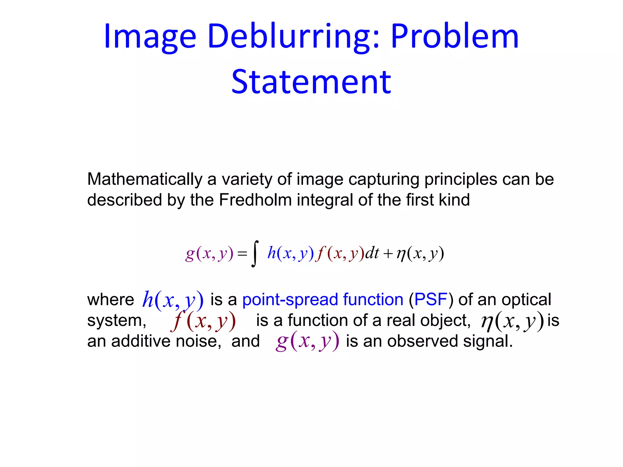
Details on image deblurring and Point-Spread Function (PSF) principles.
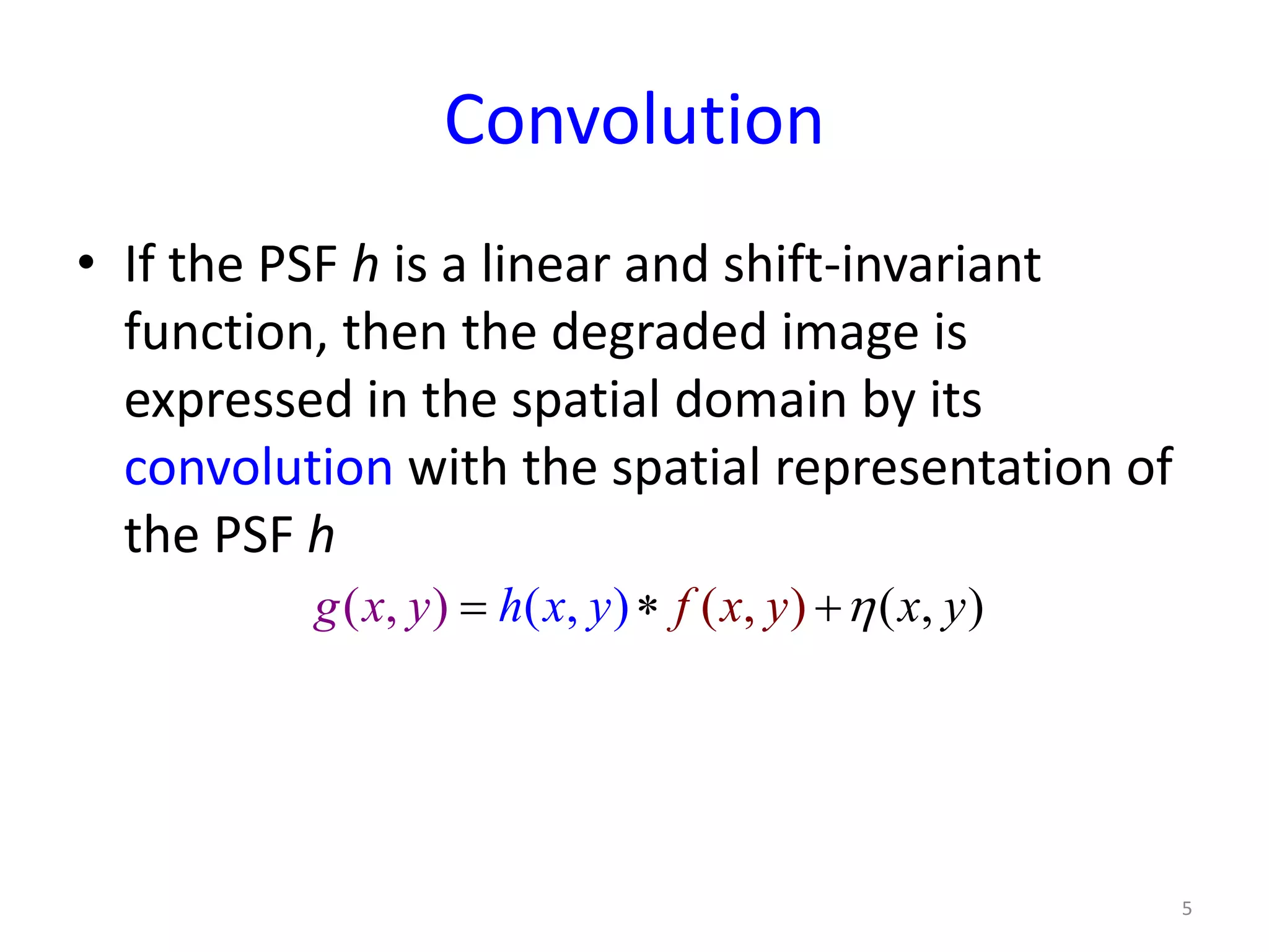
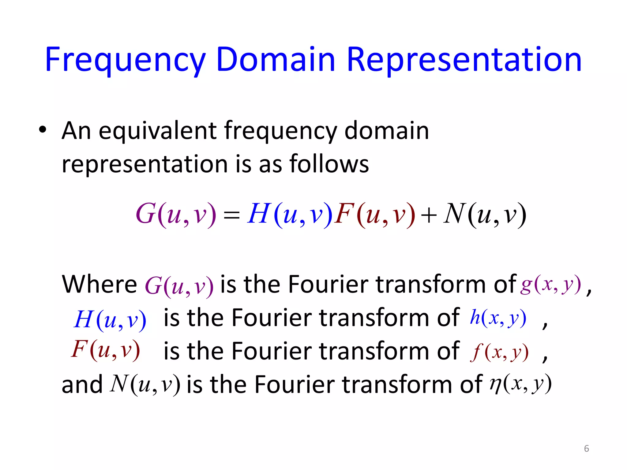
Convolution operations in spatial and frequency domains concerning image degradation.
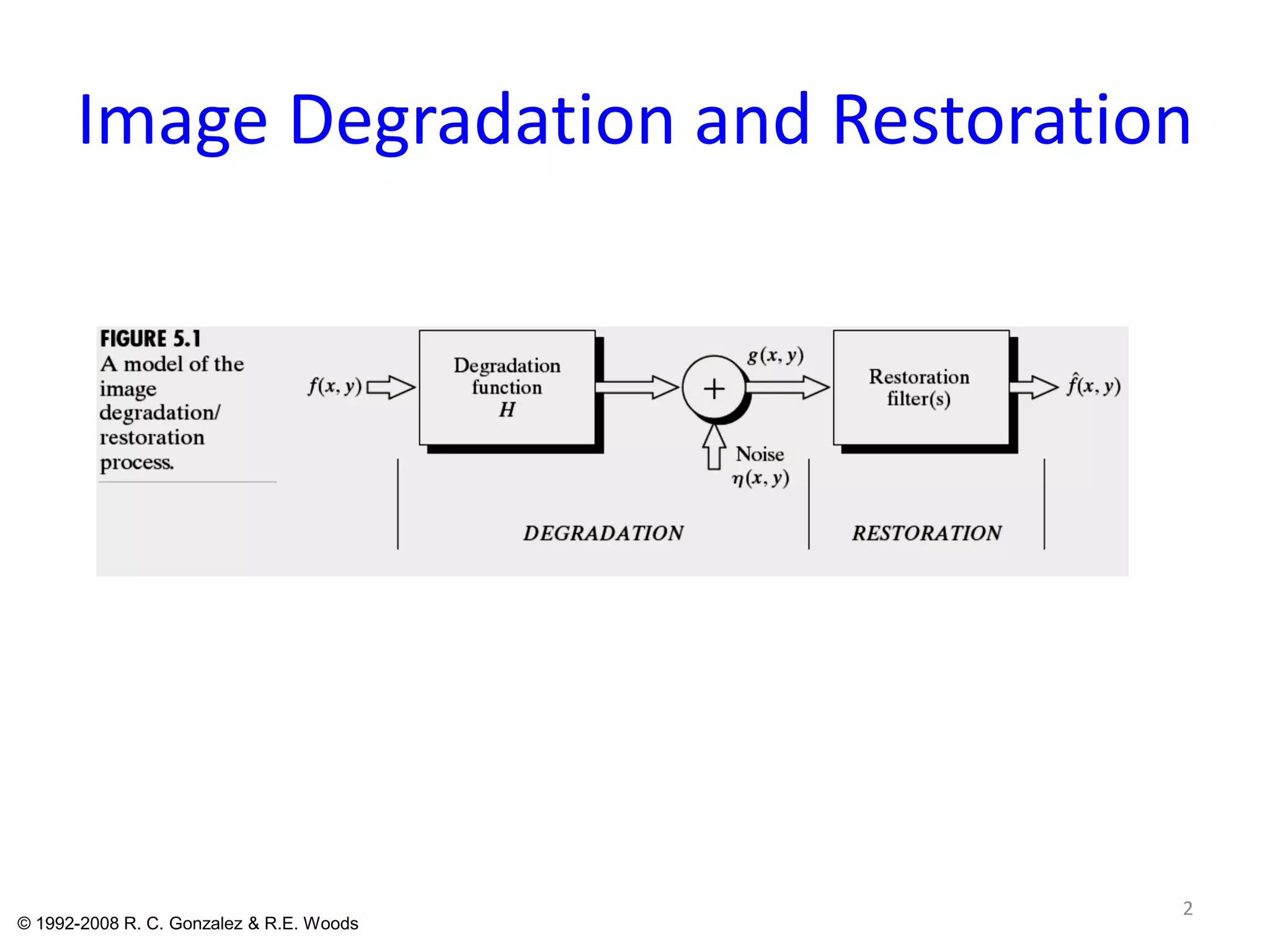
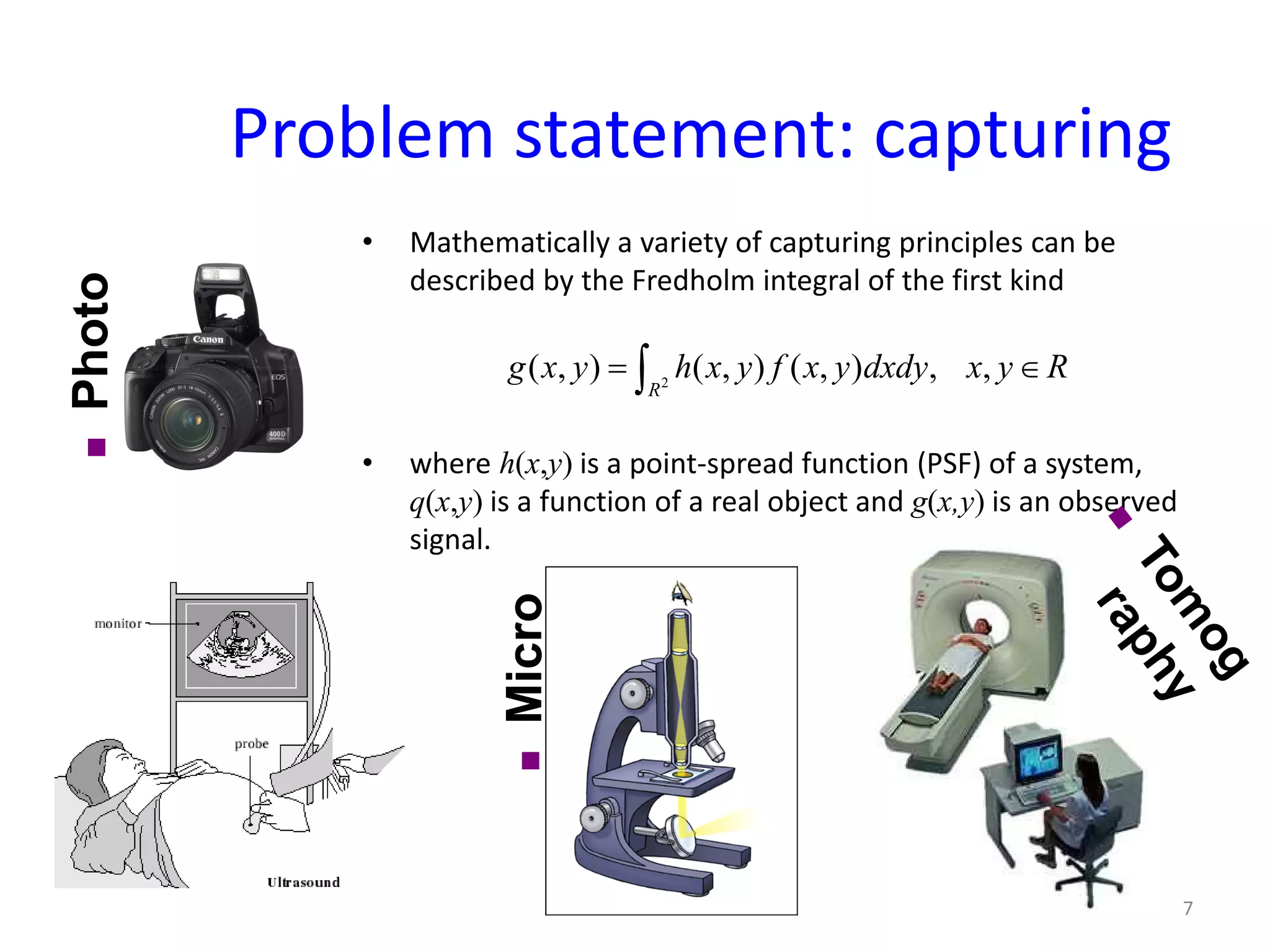
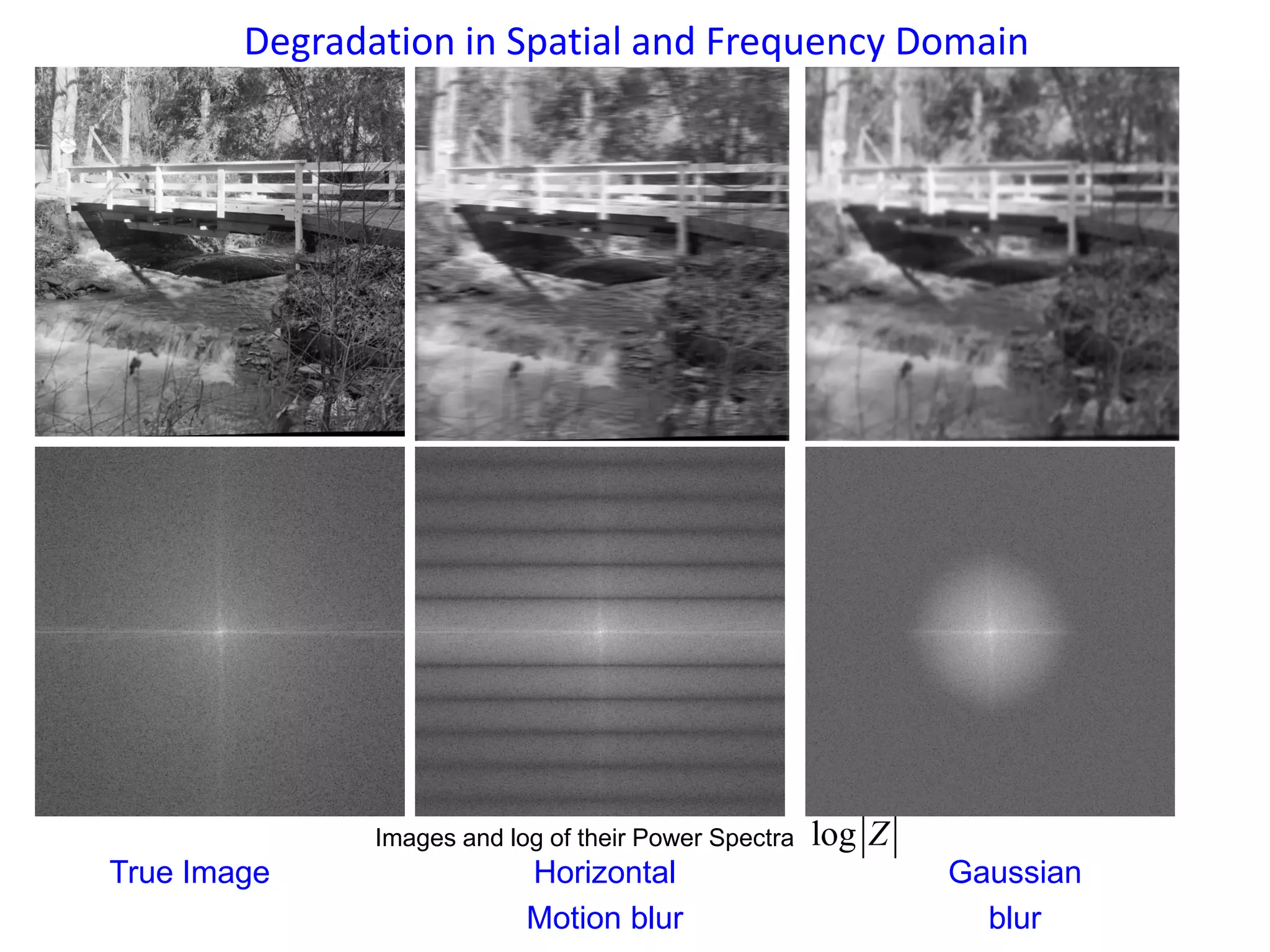
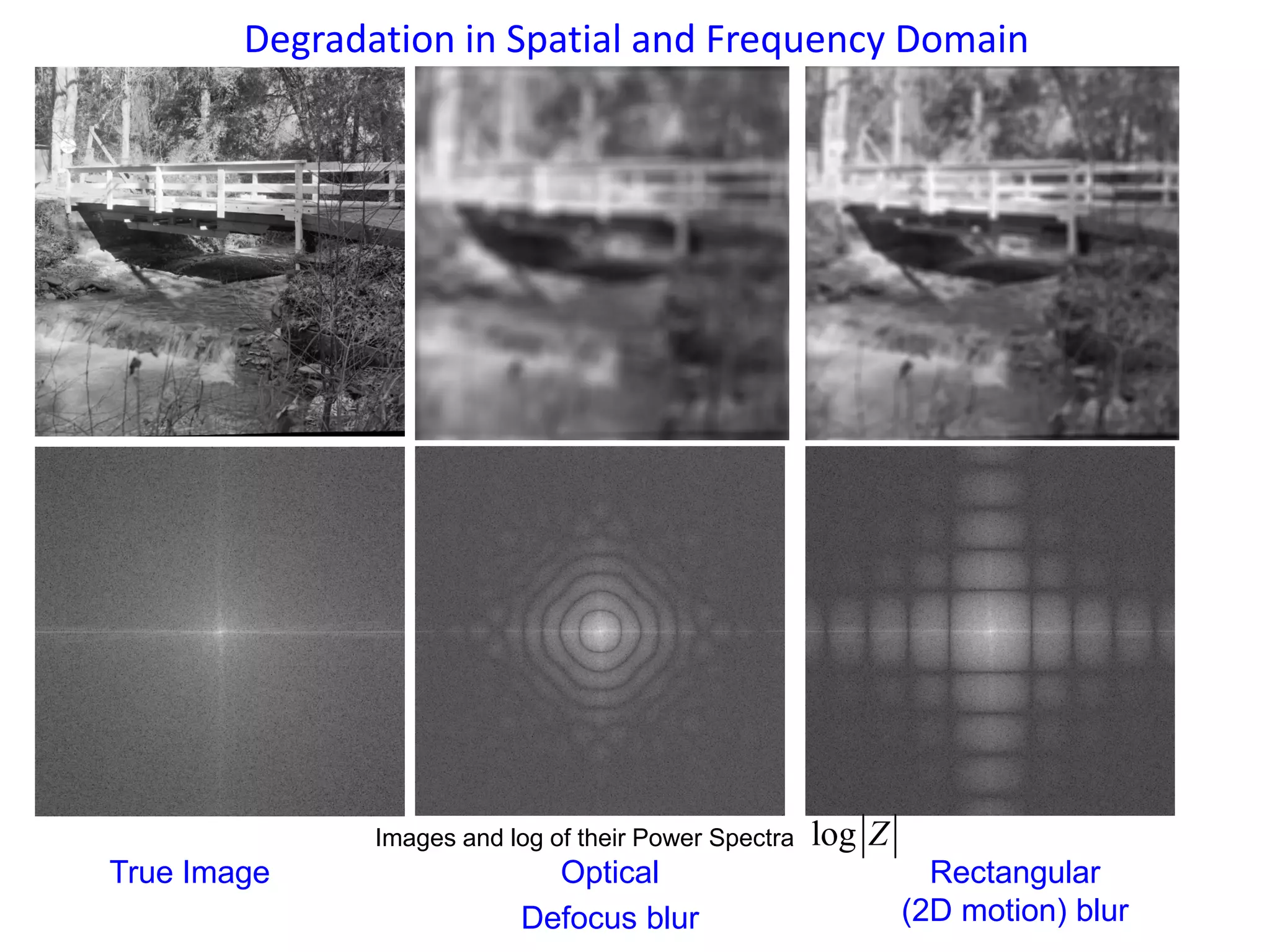
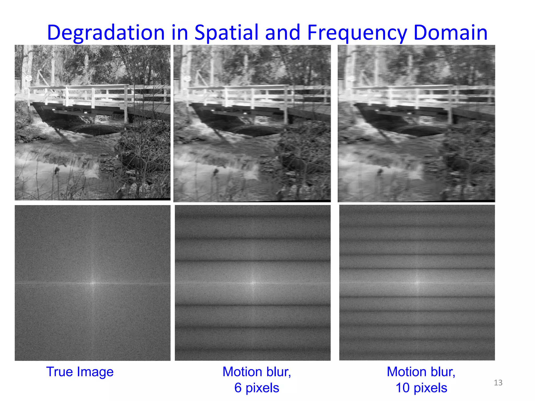
Mathematical capture principles and visual effects of blurring in spatial and frequency domains.
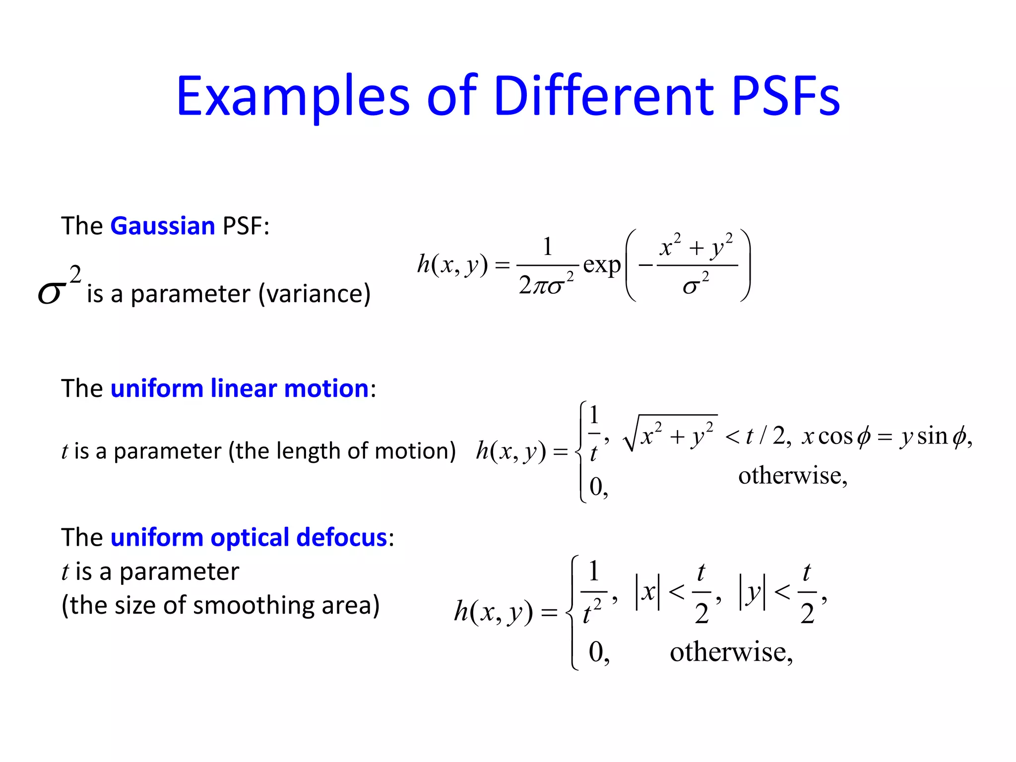
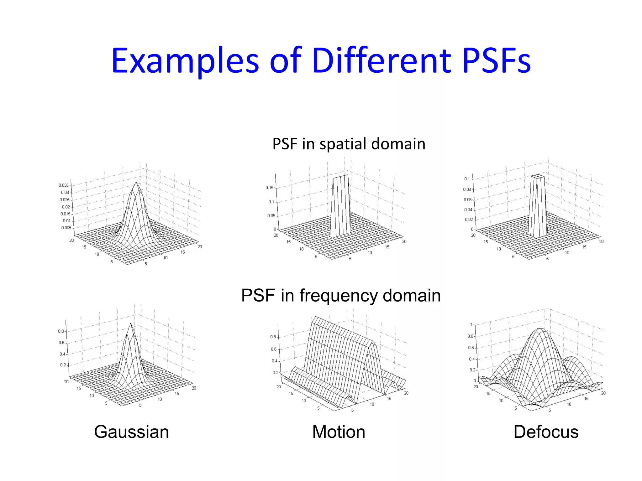
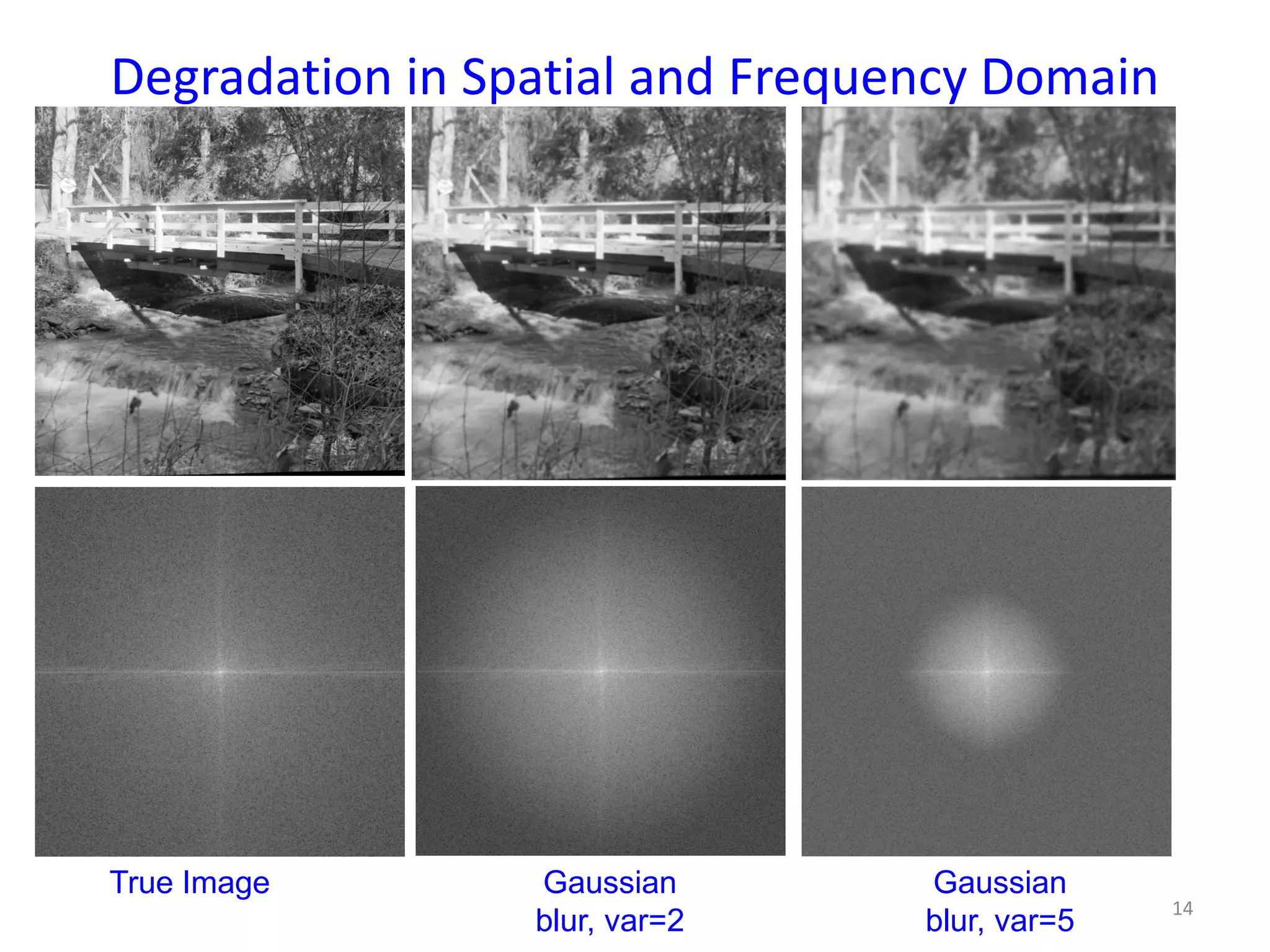
Examples of different PSFs including Gaussian and their impact on image quality.
Various types of image blurs (motion, Gaussian) and their variances affecting clarity.
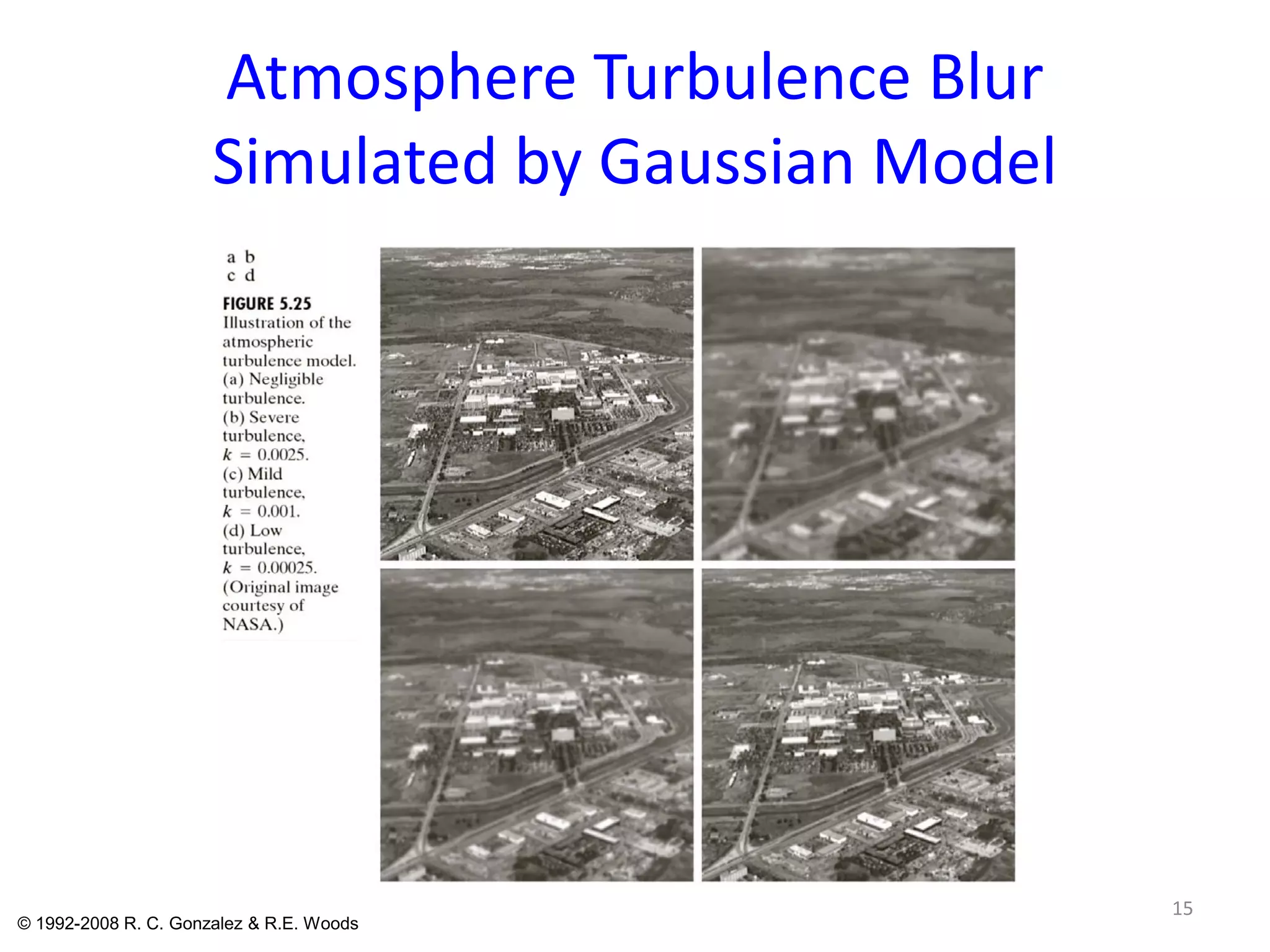
Example of image blur simulated by atmospheric turbulence using Gaussian model.
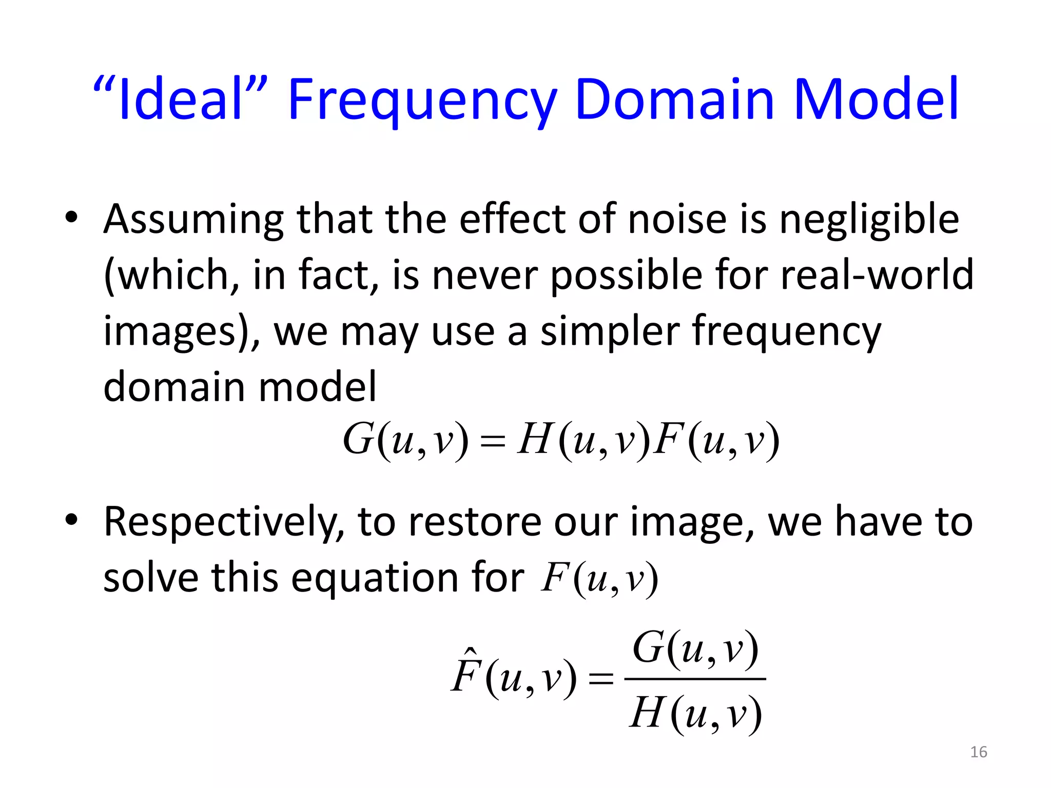
Models for restoring images in the frequency domain, focusing on noise assumptions.
Methods for solving deconvolution including exact PSF knowledge and blind deconvolution.
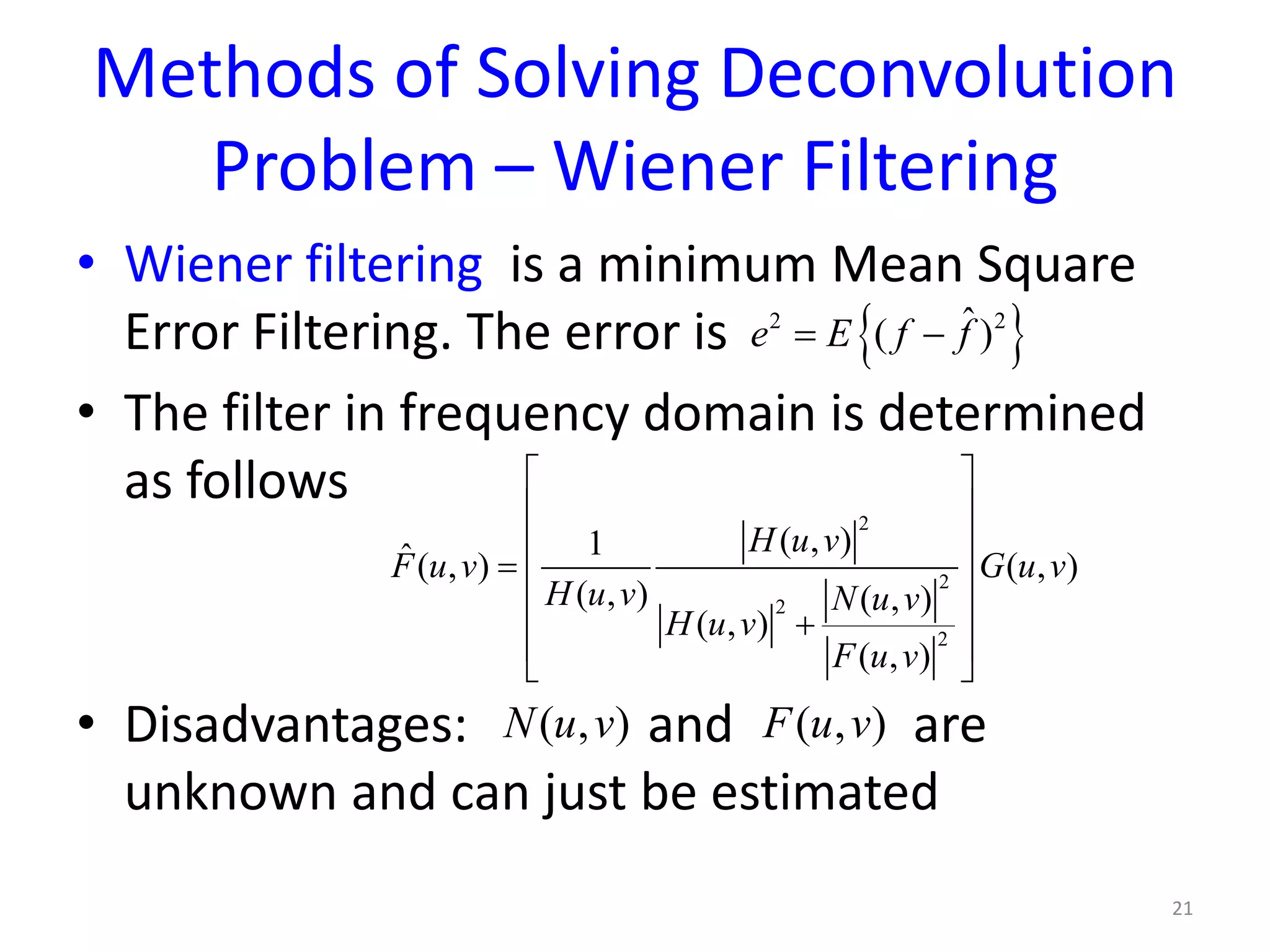
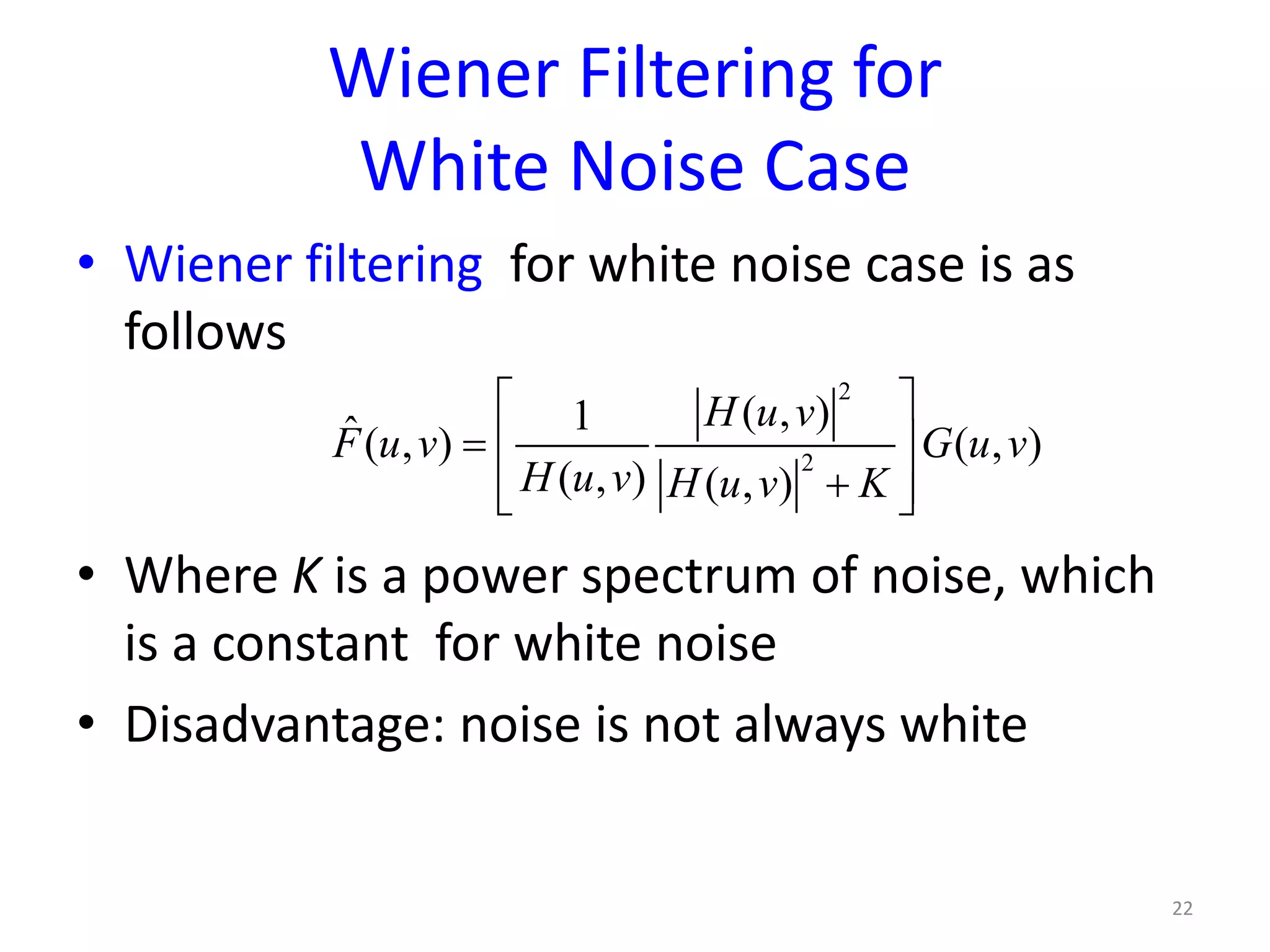
Overview of Wiener filtering in image restoration, especially for noise management.
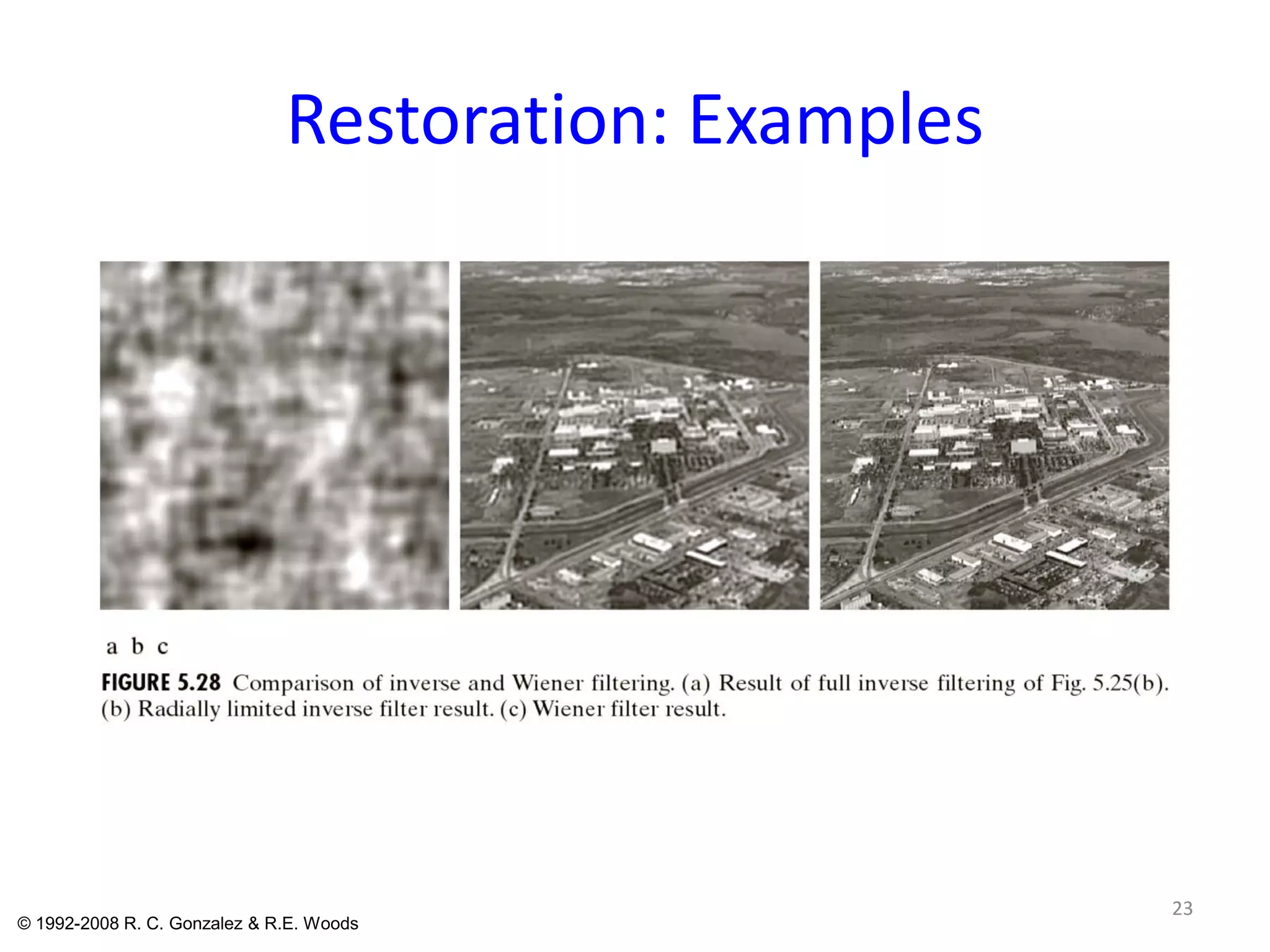
Examples showcasing the results of restoration techniques.
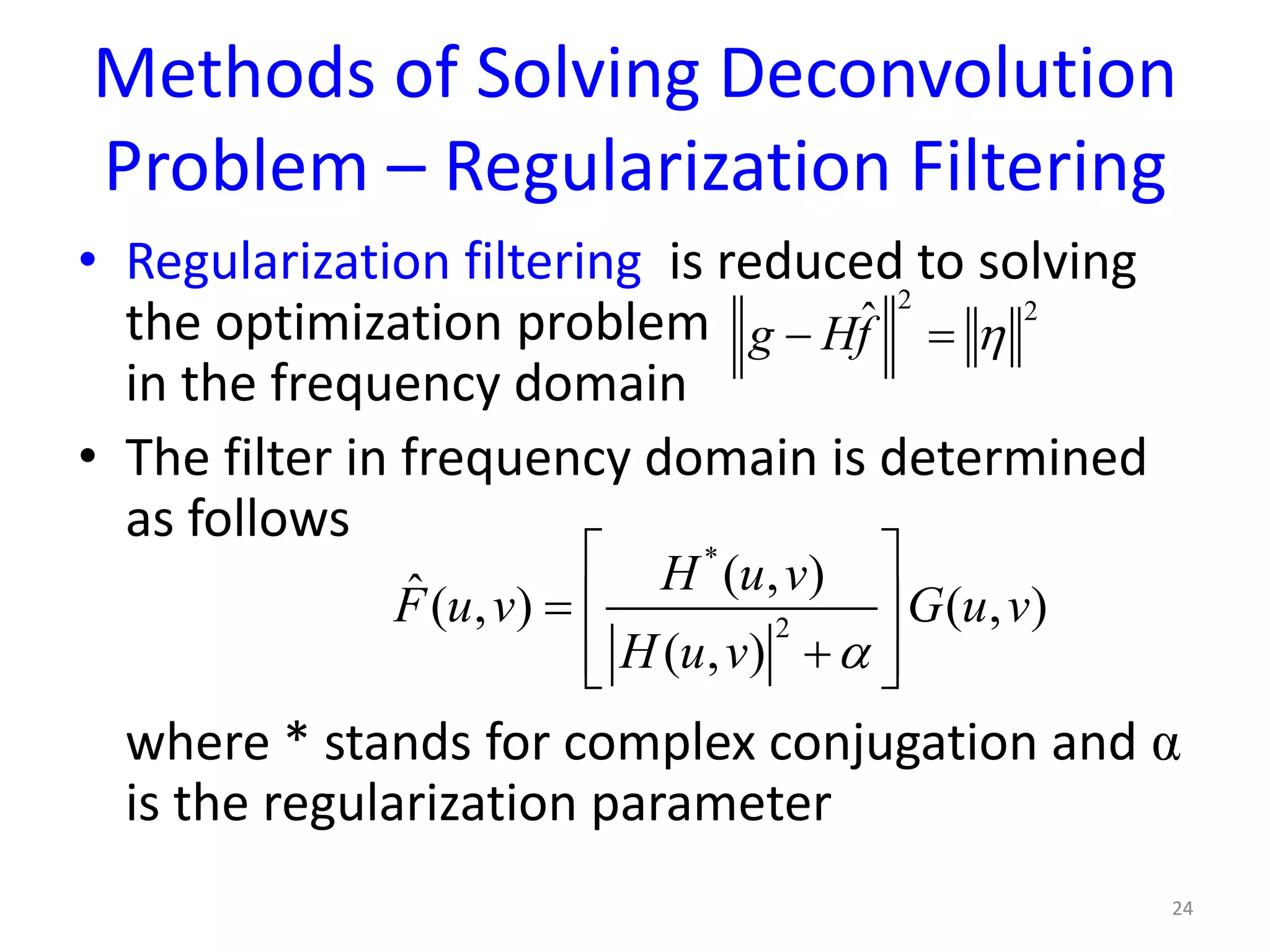
Description of regularization filtering as an optimization problem in frequency domain.
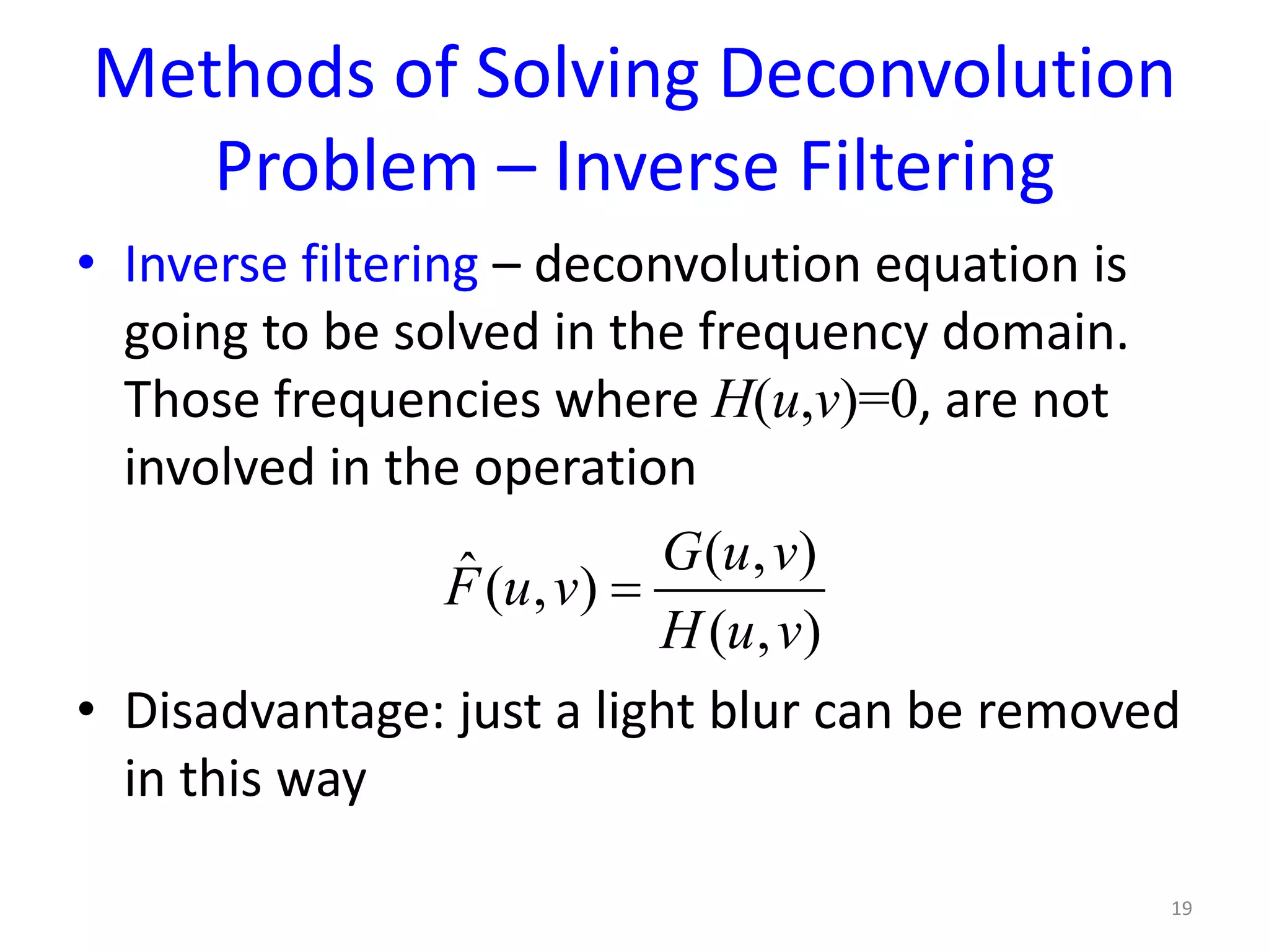
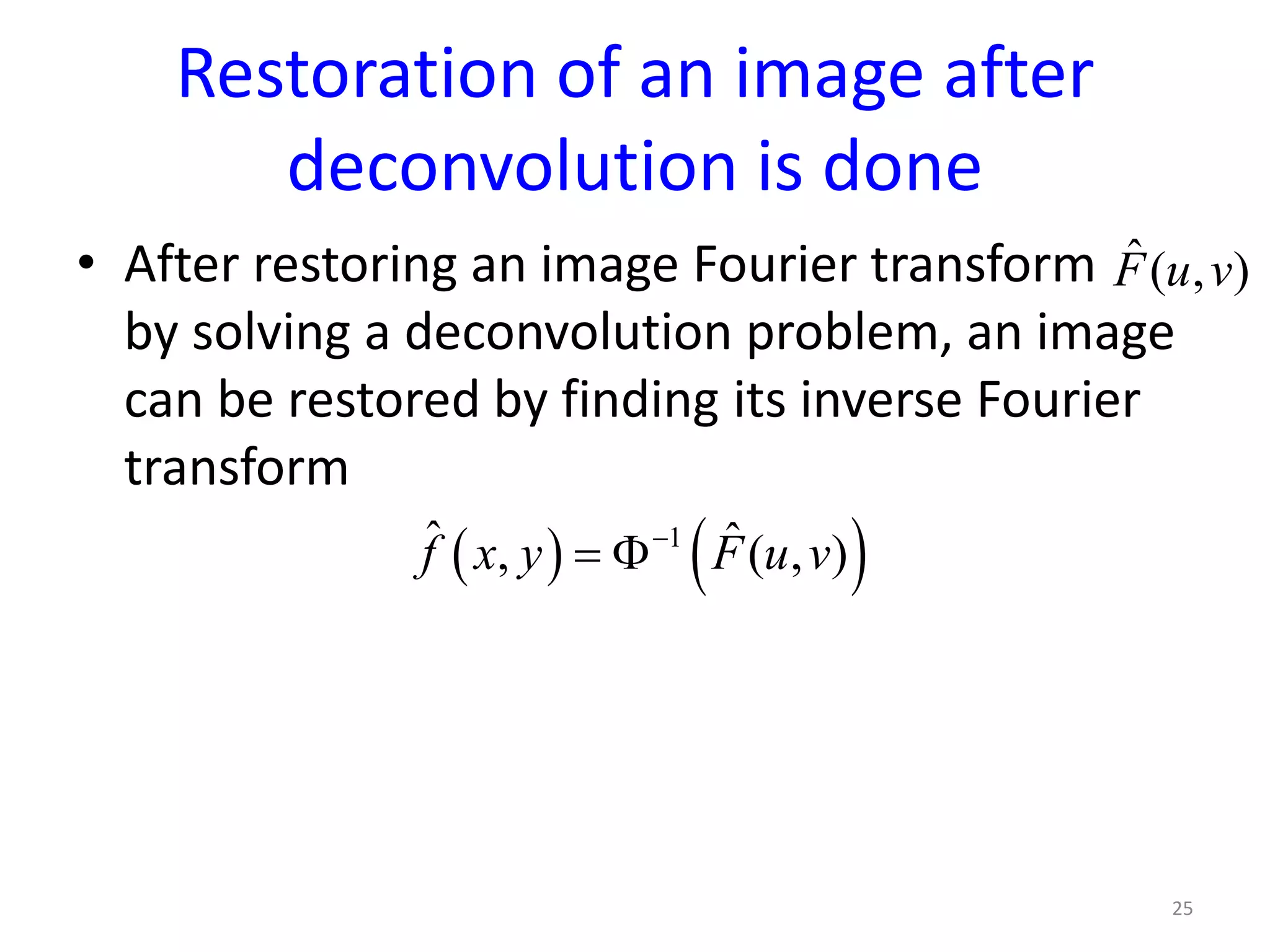
Technique of inverse Fourier transform for restoring images after deconvolution.
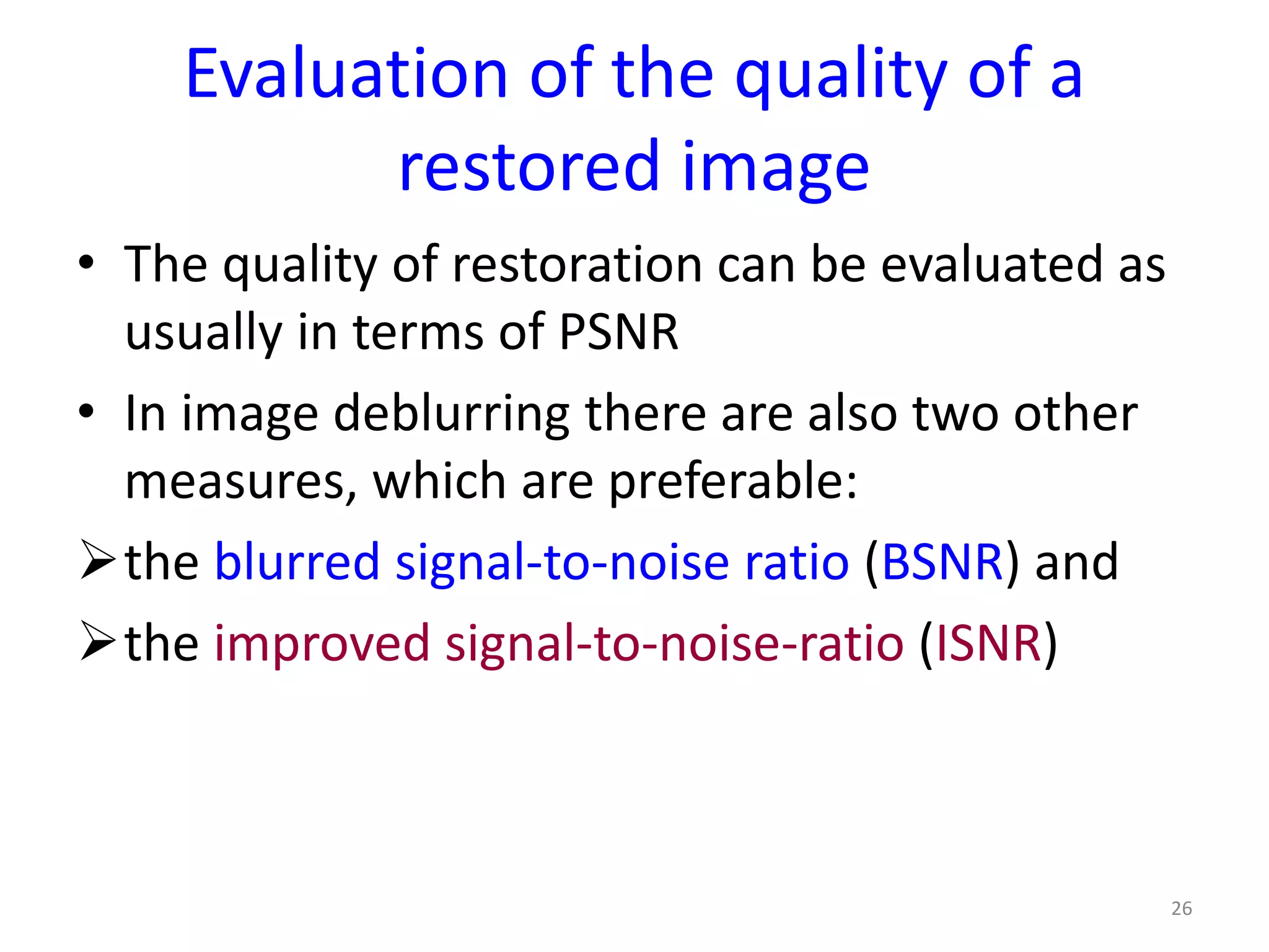
Methods for evaluating the quality of restored images including PSNR metrics.
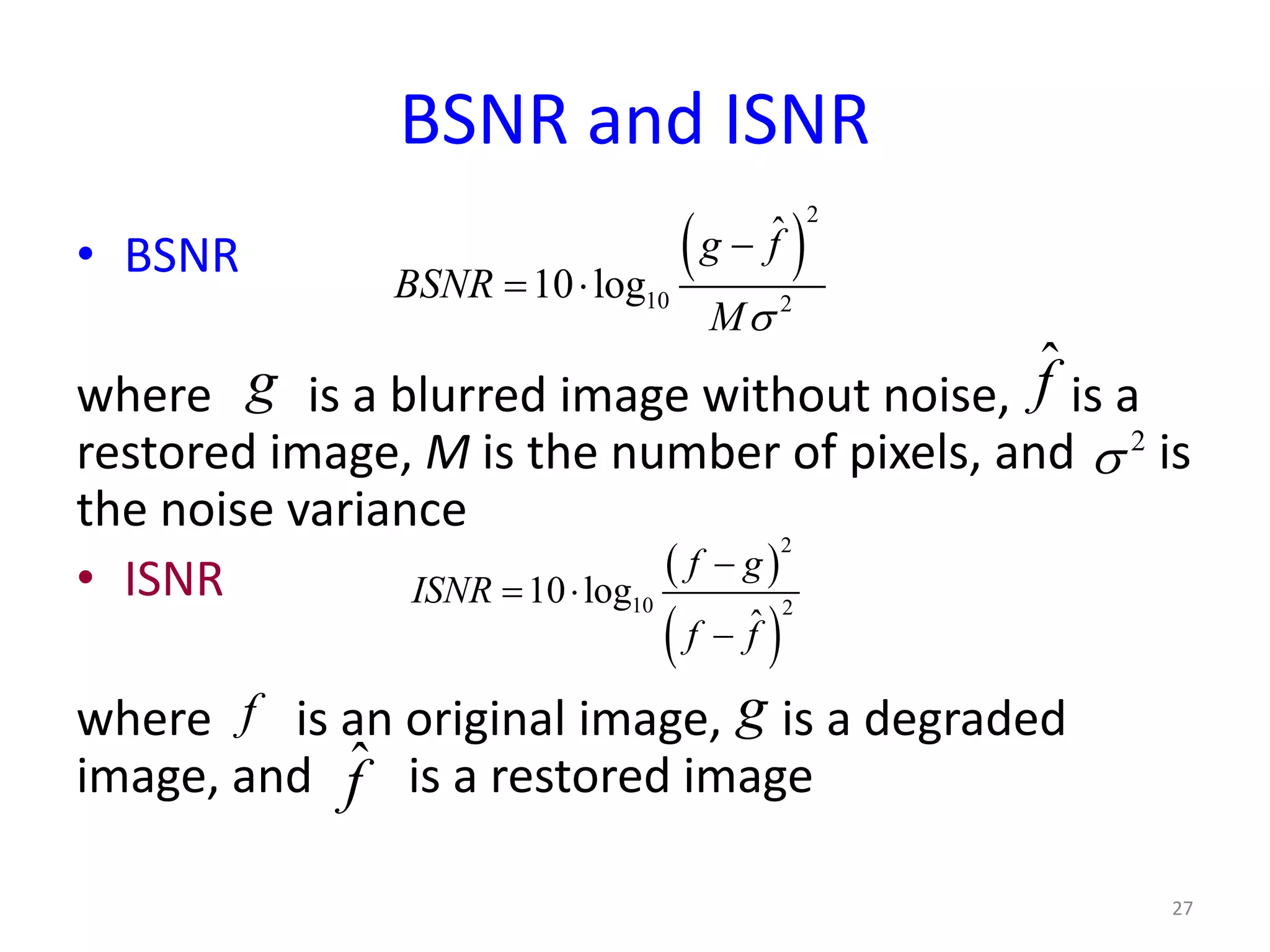
Definitions and formulas for calculating BSNR and ISNR in image restoration.


![[G4]image deblurring, seeing the invisible](https://cdn.slidesharecdn.com/ss_thumbnails/g4imagedeblurringseeingtheinvisible-120919212040-phpapp02-thumbnail.jpg?width=640&height=640&fit=bounds)