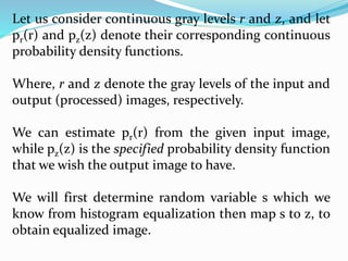
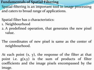
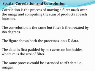
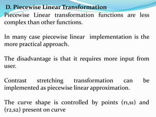
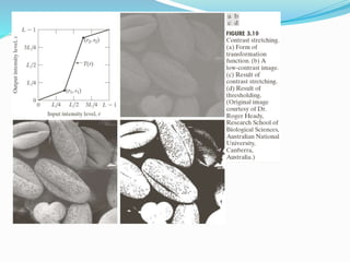
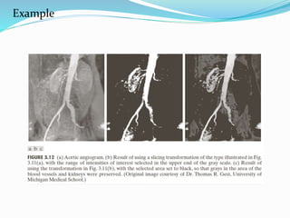
Spatial domain filtering and intensity transformations are techniques used in image processing. Spatial domain refers to the pixels that make up an image. Spatial domain techniques operate directly on pixels by applying operators to pixels and their neighbors. Common operators include averaging, median filtering, and contrast adjustments. Spatial filtering techniques include smoothing to reduce noise and sharpening to enhance edges through differentiation. Intensity transformations map input pixel values to output values using functions like logarithms, power laws, and piecewise linear approximations to modify image contrast and highlight certain intensity ranges.

1. Spatial Domain Filtering and Intensity
Transformations
Spatial domain is simply the plain containing pixels
of image.
Spatial domain techniques are more efficient
computationally and requires less processing.
Spatial domain refers to aggregate of pixels that
compose an image.

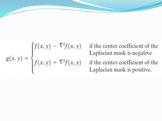
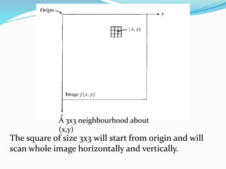
2. The spatial domain process is explained by following
expression.
g(x,y) = T[f(x,y)]
Where f(x,y) is the input image and g(x,y) is the image
at output.
T is an operator on f(x,y) defined over neighborhood
of point (x,y).
The image shows one such transformation.
An example of such transformation is image averaging.

3. A 3x3 neighbourhood about
(x,y)
The square of size 3x3 will start from origin and will
scan whole image horizontally and vertically.

4. There is no neighborhood pixels at border hence 0 or
some other intensity value is assumed.
The process just described is called as Spatial
Filtering.
The smallest neighborhood possible is 1x1 in which
new value of pixel depends on itself and in this case T
is called as Intensity Transformation Function.
Basic intensity transformation functions include
image negatives, log transform etc.

5. Example of contrast stretching and
thresholding

6. In image intensity transformation the relation between input
and output is given by
s= T(r)
r is pixel before processing and s is output pixel value.
A. Image Negatives
The relation between input and output is given by
s=L-1-r
It produces equivalent of image negative.
It is used for enhancing white/gray details in dark region.

8. B. Log Transformation
s= clog(1+r)
Where c is constant and r >=0.
It maps narrow range of low level in wide range of
output levels and vice versa.
It expands dark pixel value while compressing higher
pixel values.
Inverse log transforms is also there which does the
opposite task of log transformation.
Example in Fourier transform.

9. C. Power Law Transformation
As name suggests, it has exponential relation between
input and output.
s = crγ
Or some times as s = c(r+eps)γ
It is better than log transform as more possibilities at
output are present depending on value of gamma.
The term gamma correction used in TV industry
performs power law transformation.

14. D. Piecewise Linear Transformation
Piecewise Linear transformation functions are less
complex than other functions.
In many case piecewise linear implementation is the
more practical approach.
The disadvantage is that it requires more input from
user.
Contrast stretching transformation can be
implemented as piecewise linear approximation.
The curve shape is controlled by points (r1,s1) and
(r2,s2) present on curve

16. Consider the piecewise linear function for following
three cases
1. r1 = s1 and r2 = s2
2. r1 = r2 and s1 = 0 and s2 = L-1
3. r1<r2 and s1<s2
Intensity Level Slicing
Slicing is done to highlight certain range of
intensities in an image. This is done by two
approaches

17. The first approach in intensity slicing could be to
display range of interest in one colour and all other
intensity by other.
In second approach colour of range of intensities is
changed and only and other intensities remain as it is

18. Example

19. Bit Plane Slicing
We can make a binary image by using singke bit of every
pixel.
If L=256 every pixel would contain 8 bits thus we can
make 8 binary images starting from LSB to MSB.
By doing this we can highlight contribution of specific
bits in an image.

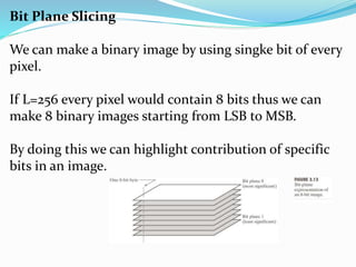
22. Histogram Processing
The histogram of a digital image with intensity levels
in intensity range [0,L-1]is a discrete function h(rk) =
nk where rk is the kth intensity value and and nk is the
number of pixels in the image with intensity rk.
Histogram can be normalized by dividing each of its
components by total number of pixels present in the
image.
If MN is total number of pixels where M is the number
of rows in the image and N is the coloumns.

23. Then normalized histogram is given by:
p(rk) = nk/MN
It can be said that p(rk) is the estimate of the
probability of occurrence of intensity level rk.
Histograms forms the basis of numerous spatial
domain processing techniques.
Histogram can be used for image enhancements also
histogram equalization is one of an example of image
enhancement by histogram processing.

25. Histogram Equalization
Let the variable r represent the gray levels of the image
to be enhanced.
We assume that the transformation function
T(r) satisfies the following conditions:
(a)T(r) is single-valued and monotonically increasing
in the interval 0<= r <= 1; and
(b) 0 <=T(r) <=1 for 0 <=r <=1.

27. Let us discuss the histogram Equalization in detail.
First we shall discuss it for continuous pdf and then
we will extend it to discrete pdf case.

28. Example
Consider 64x64 pixel
3bit image
L=8 and L-1 =7 with
specification in
adjoining table

30. Histogram Matching
Histogram equalization process automatically
determines the function which generates an image
with uniform histogram at the output.
In many cases the uniform histogram is not the
required output and we want a histogram to acquire a
specific shape or distribution at the output.
The method used to generate a processed image that
has a specified histogram is called histogram matching
or histogram specification.

31. Let us consider continuous gray levels r and z, and let
pr(r) and pz(z) denote their corresponding continuous
probability density functions.
Where, r and z denote the gray levels of the input and
output (processed) images, respectively.
We can estimate pr(r) from the given input image,
while pz(z) is the specified probability density function
that we wish the output image to have.
We will first determine random variable s which we
know from histogram equalization then map s to z, to
obtain equalized image.

32. Fundamentals of Spatial Filtering
Spatial filtering is an important tool in image processing
and caters to broad range of applications.
Spatial filter has 2 characteristics:
1. Neighbourhood
2. A predefined operation, that generates the new pixel
value.
The coordinates of new pixel is same as the center of
neighbourhood.
At each point (x, y), the response of the filter at that
point i.e. g(x,y) is the sum of products of filter
coefficients and the image pixels encompassed by the
image.

33. g(x,y) = w(-1,-1)*f(x-1,y-1) + w(-1,0)*f(x-1,y) +
…w(0,0)*f(x,y) + …. w(1,1)*f(x+1,y+1)

34. The coefficient w(0, 0) coincides with image value f(x,
y), indicating that the mask is centered at (x, y) when
the computation of the sum of products takes place.
For a mask of size m*n, it is assumed that m=2a+1 and
n=2b+1, where a and b are nonnegative integers.
It means that masks are of odd sizes, with the smallest
meaningful size being 3*3.

35. Spatial Correlation and Convolution
Correlation is the process of moving a filter mask over
the image and computing the sum of products at each
location.
The convolution is the same but filter is first rotated by
180 degrees.
The figure shows both the processes on 1 D data.
The data is first padded by m-1 zer0s on both sides
where m is the size of filter.
The same process could be extended to 2D data i.e.
images.

38. 2D Correlation
2D Convolution
a =? b = ?

39. Smoothing filters are used for blurring and noise
reduction.
The implemented filter could be linear or non linear.
The linear filter is one in which the relationship between
input and output is linear.
Similarly, non linear filters can be implemented.
Example of linear filters is: Averaging Filter
Example of Non - linear filters is: Median Filter
Smoothing Spatial Filters

40. Where blurring is implemented in preprocessing tasks to
remove small details from an image prior to large object
extraction.
The output of a smoothing (averaging or lowpass) linear
spatial filter is the average of the pixels contained in the
neighborhood of the filter mask.
By replacing the value of every pixel in an image by the
average of the intensity levels in the neighborhood
defined by a filter mask, the resulting image will have
reduced “sharp” transitions in intensities.

41. As random noise typically corresponds to such
transitions, we can achieve denoising.
However, edges are often characterized by sharp
intensity transitions, so smoothing linear filters may
have the undesirable side effect on edges.
Examples of such masks:
1) A box filter – spatial averaging filter 3x3
2) Weighted average filter attempt to reduce blurring

42. The second mask, shown in Figure is called weight
average, thus giving more importance (weight) to some
pixels at the expense of others.
The general implementation for filtering an M ×N image
with a weighted averaging filter of size m ×n is given by
the expression

45. Order-statistic (nonlinear) filters
Order-statistic filter are nonlinear spatial filters.
There response is based on ordering (Ranking) the
pixels in the neighborhood and then replacing the value
of the center pixel by the value determined by the
ranking result.
The median filters are quite effective against the impulse
noise (salt-and-pepper noise).
Ex: the 3x3 neighborhood has values (10, 20, 20, 20,15,
20, 100, 25, 20). These values are ranked as (10, 15, 20, 20,
20, 20, 20, 25, 100). The median will be 20.

47. Sharpening Spatial Filters
Sharpening highlight transitions in intensity.
It is used in areas like electronic printing, medical
imaging, industry and military applications.
Image smoothing requires blurring of images which
performs averaging operation which is analogous to
integration.
So, sharpening operation can be accomplished by spatial
differentiation.
The image differentiation enhances edges and other
discontinuities and deemphasizes areas with slowly
varying intensities.

48. First and Second Order Derivative
The derivatives of a digital function are defined in terms
of differences. There are various ways to define these
differences.
Following are the condition that a first order derivative
must fulfill:
a. must be zero in flat segments (areas of constant gray-level
values)
b. must be nonzero at the onset of a gray-level step or ramp and
c. must be nonzero along ramps.
Similarly a second order derivative must fulfill following
condition.
a. must be zero in flat areas
b. must be nonzero at the onset and end of a gray-level step or
ramp
c. must be zero along ramps of constant slope.

49. A basic definition of the first-order derivative of a one-
dimensional function f(x) is the difference given by:
Similarly, a second-order derivative can be defined as the
difference

52. First-order derivatives generally produce thicker edges in
an image.
Second-order derivatives have a stronger response to fine
detail, such as thin lines and isolated points.
First order derivatives generally have a stronger response
to a gray-level step.
Second order derivatives produce a double response at
step changes in gray level.
In most applications, the second derivative is better
suited than the first derivative for image enhancement
because of its ability to enhance fine detail and simpler
implementation.

53. The Laplacian
The Laplacian is a two-dimensional, second order
derivatives for image enhancement.
The Laplacian is an isotropic derivative operator , which,
for a function (image) f(x, y) of two variables, is defined
as:
The filter mask created by Laplacian generates isotropic
filters, which means their response is independent of the
direction of the discontinuities in the image.
The Laplacian are the simplest isotropic derivative
operator. The word isotropic denotes that generated filter
is rotation invariant.