Download as PDF, PPTX

![Inverse Filtering
• The simplest approach to restoration is direct inverse filtering, where
we compute an estimate, 𝐹 𝑢, 𝑣 , of the transform of the original
image simply by dividing the transform of the degraded image, G(u, v),
by the degraded function:
𝐹 𝑢, 𝑣 =
𝐺(𝑢, 𝑣)
𝐻(𝑢, 𝑣)
Substituting the RHS of frequency domain representation of
the model of image degradation/reconstruction we get:
𝐹 𝑢, 𝑣 = 𝐹 𝑢, 𝑣 +
𝑁(𝑢, 𝑣)
𝐻(𝑢, 𝑣)
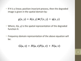
This equation tells that, even if we know the degradation function we
cannot recover the un-degraded image [F(u, v)] exactly because N(u, v) is
not known.
If degradation function has zero or very small value then the ratio could
easily dominate the result. 16](https://image.slidesharecdn.com/imagereconstruction-210417050320/85/Image-restoration-and-reconstruction-16-320.jpg)
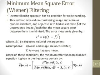
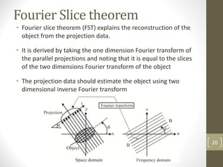
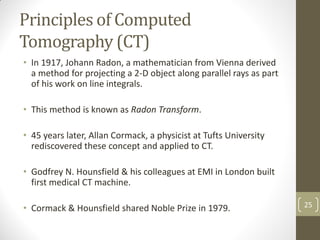
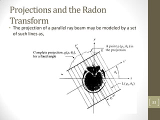
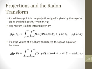
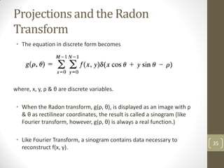
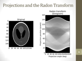
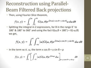
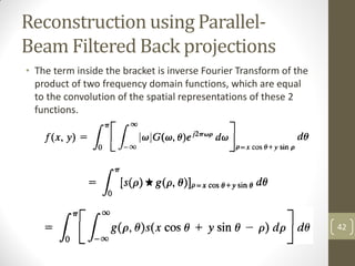
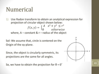
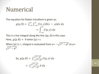
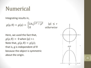
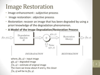
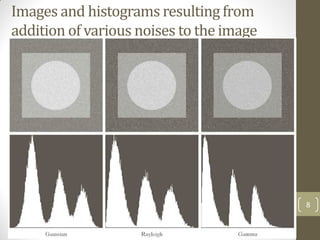
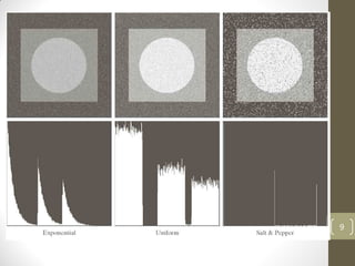
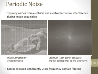
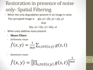
The document discusses image restoration and reconstruction techniques. It covers topics like image restoration models, noise models, spatial filtering, inverse filtering, Wiener filtering, Fourier slice theorem, computed tomography principles, Radon transform, and filtered backprojection reconstruction. As an example, it derives the analytical expression for the projection of a circular object using the Radon transform, showing that the projection is independent of angle and equals 2Ar√(r2-ρ2) when ρ ≤ r.