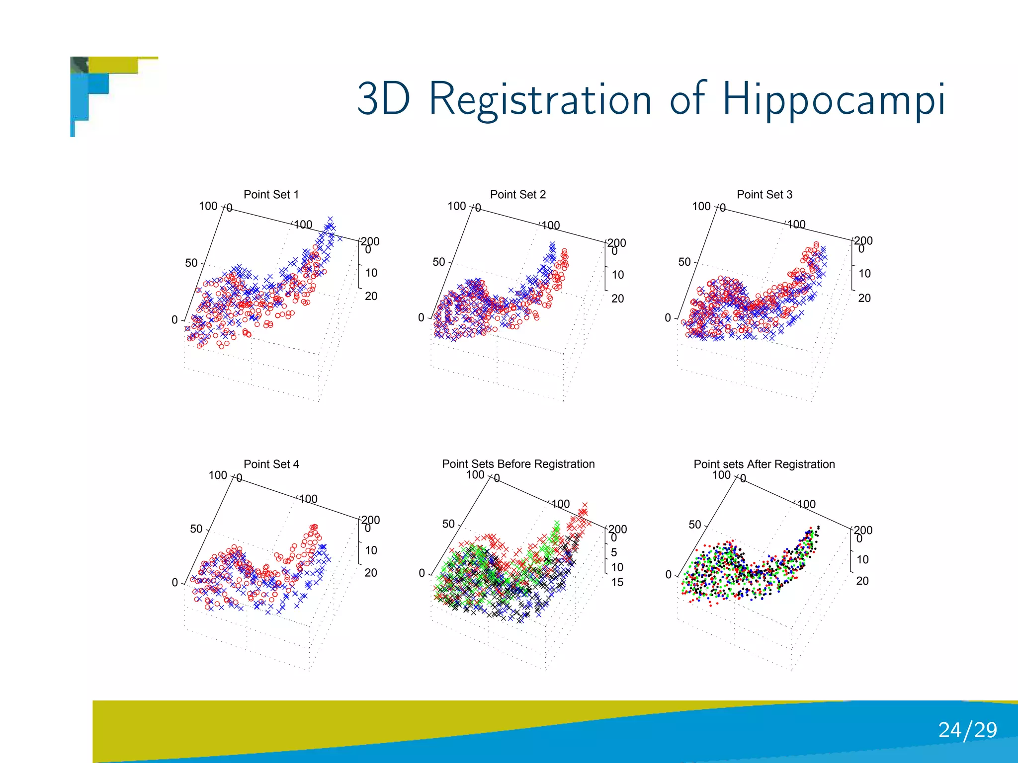
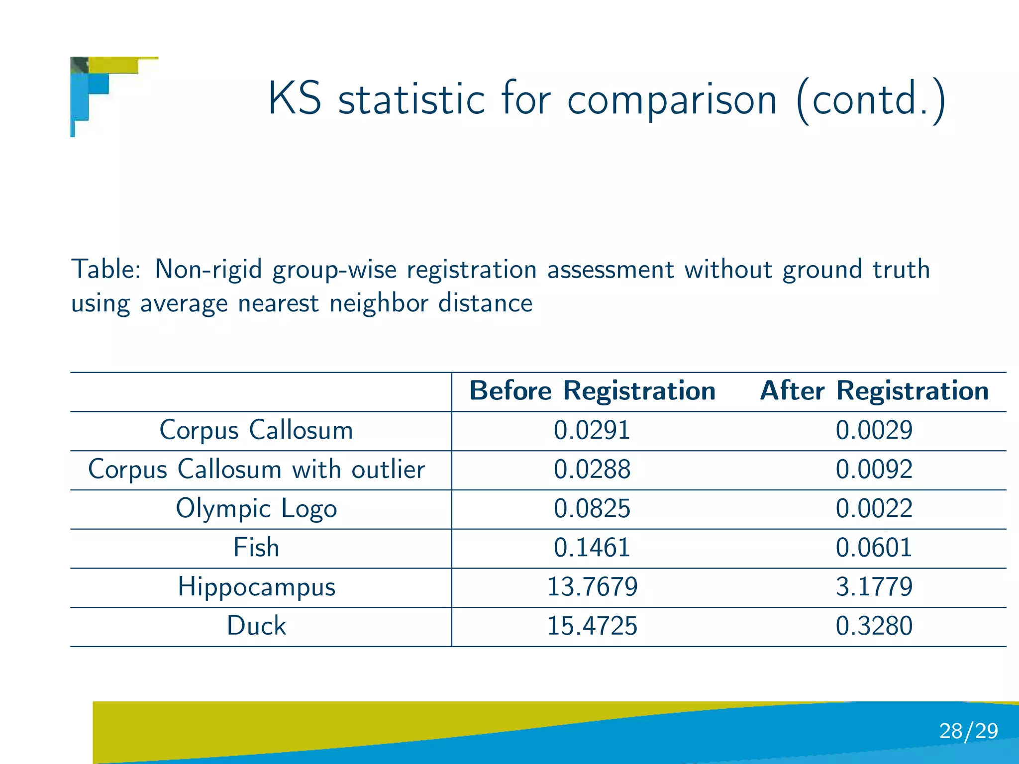
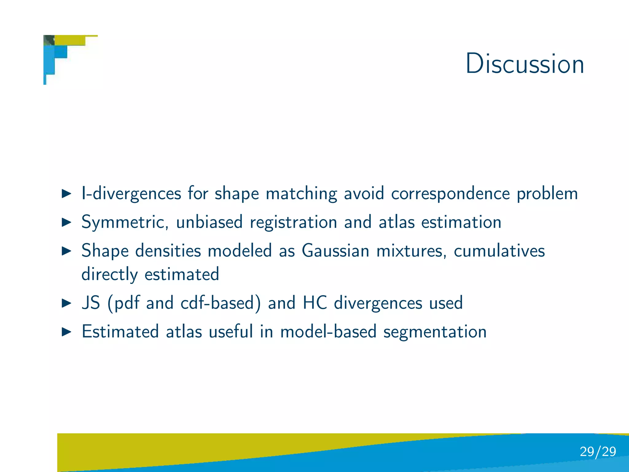
The document discusses using divergence measures like the Jensen-Shannon divergence to align multiple point sets represented as probability density functions. It motivates using the JS divergence by modeling point sets as mixtures of density functions, and shows how the likelihood ratio between models leads to the JS divergence. It then formulates the problem of group-wise point set registration as minimizing the JS divergence between density functions, combined with a regularization term. Experimental results on aligning multiple 3D hippocampus point sets are also presented.

1. A vne
da cd
Ifr t nT e r i
nomai h oyn
o
C P “ aN t e”
VRi n us l
hl
CP
VR
T ti
u rl
oa J n 1 -82 1
u e 31 0 0
S nFa c c ,A
a rn i oC
s
Shape Matching with I-divergences
Anand Rangarajan

2. Shape Matching with I-Divergences
Groupwise Point-set Pattern Registration
Given N point-sets, which are denoted by {X p , p ∈ {1, ..., N}}, the
task of multiple point pattern matching or point-set registration is to
recover the spatial transformations which yield the best alignment of
all shapes.
2/29

3. Problem Visualization
3/29

4. Problem Visualization
3/29

5. Group-wise Point-set Registration
Principal Technical Challenges
Solving for nonrigid deformations between point-sets with
unknown correspondence is a difficult problem.
How do we align all the point-sets in a symmetric manner so
that there is no bias toward any particular point-set?
4/29

6. From point-sets to density functions
5/29

7. From point-sets to density functions
5/29

8. Group-wise Point-set Registration
From point-sets to density functions
Point sets are represented by probability density functions.
Intuitively, if these point sets are aligned properly, the
corresponding density functions should be similar.
6/29

9. Group-wise Point-set Registration
From point-sets to density functions
Point sets are represented by probability density functions.
Intuitively, if these point sets are aligned properly, the
corresponding density functions should be similar.
Question: How do we measure the similarity between multiple
density functions?
6/29

10. Divergence Measures
Kullback-Leibler divergence
ˆ
p(x)
DKL (p q) = p(x) log dx
q(x)
where p(x), q(x) are the probability
density functions.
7/29

11. Divergence Measures
Kullback-Leibler divergence J divergence
ˆ Given two probability density
p(x) function p and q, the symmetric KL
DKL (p q) = p(x) log dx
q(x) divergence is defined as:
where p(x), q(x) are the probability 1
J(p, q) = (DKL (p q) + DKL (q p))
density functions. 2
7/29

12. Motivating the JS divergence
Modeling two shapes
X Y
N1 K1 N2 K2
(1) 1 (1) (2) 1 (2)
p(X |θ )= p(Xi |θa ), p(Y |θ )= p(Yj |θb )
K1 K2
i=1 a=1 j=1 b=1
8/29

13. Motivating the JS divergence
Modeling the overlay of two shapes with identity of origin
X Y
p(X ∪ Y |θ(1) , θ(2) ) = p(X |θ(1) )p(Y |θ(2) )
8/29

14. Motivating the JS divergence
Modeling the overlay of two shapes without identity of origin
Z
N1 N2
p(Z |θ(1) , θ(2) ) = p(Z |θ(1) ) + p(Z |θ(2) )
N1 + N2 N1 + N2
8/29

15. Likelihood Ratio
Which generative model do you prefer? The union of disparate
shapes where identity of origin is preserved or one combined
shape where the identity of origin is suppressed.
Likelihood ratio:
N1 (1) N2 (2)
p(Z |θ(1) , θ(2) ) N1 +N2 p(Z |θ ) + N1 +N2 p(Z |θ )
log Λ = log =
p(X ∪ Y |θ(1) , θ(2) ) p(X |θ(1) )p(Y |θ(2) )
Z is understood to arise from a convex combination of two
mixture models p(Z |θ(1) ) and p(Z |θ(2) ) where the weights of
each mixture are proportional to the number of points N1 and
N2 in each set.
Weak law of large numbers leads to Jensen-Shannon divergence.
9/29

16. JS Divergence for multiple shapes
JS-divergence of shape densities
JSπ (P1 , P2 , ..., Pn ) = H( π i Pi ) − πi H(Pi ) (1)
where π = {π1 , π2 , ..., πn |πi > 0, πi = 1} are the weights of the
probability densities Pi and H(Pi ) is the Shannon entropy.
10/29

17. Atlas estimation
Formulation using JS-divergence
N
JSβ (P1 , P2 , ..., PN ) + λ ||Lf i ||2
i=1
N
=H( β i Pi ) − βi H(Pi ) + λ ||Lf i ||2 .
i=1
f i is the deformation function corresponding to point set X i ;
Pi = p(f i (X i )) is the probability density for deformed point-set.
11/29

18. Multiple shapes: JS divergence
JS divergence in a hypothesis testing framework:
Construct a likelihood ratio between i.i.d. samples drawn from a
mixture ( a πa Pa ) and i.i.d. samples drawn from a
heterogeneous collection of densities (P1 , P2 , ..., PN ).
The likelihood ratio is then
M N
k=1 a=1 πa Pa (xk )
Λ= N Na
.
a
a=1 ka =1 Pa (xka )
Weak law of large numbers gives us the JS-divergence.
12/29

19. Group-wise Registration Results
Experimental results on four 3D hippocampus point sets.
13/29

20. Shape matching via CDF I-divergences
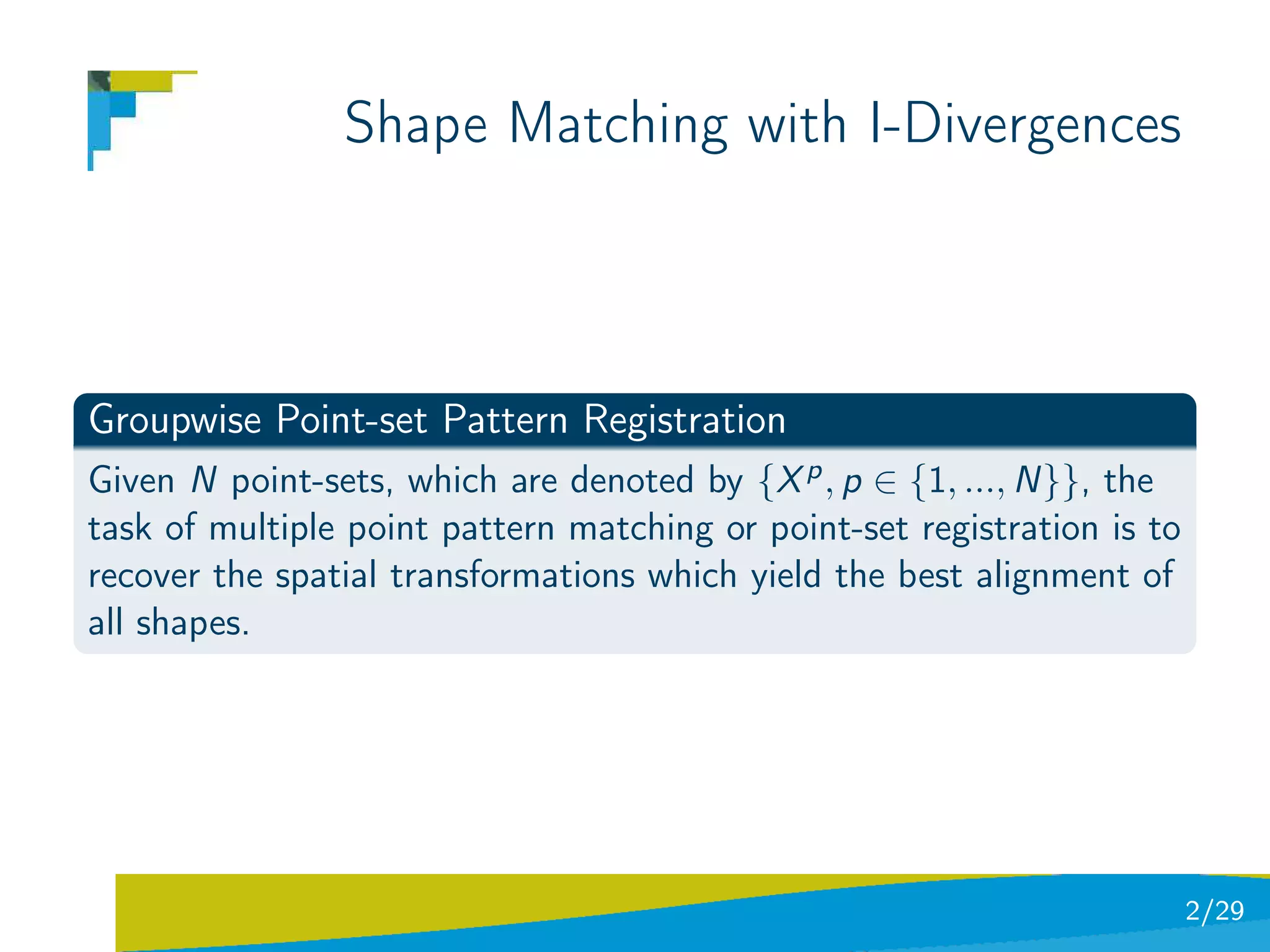
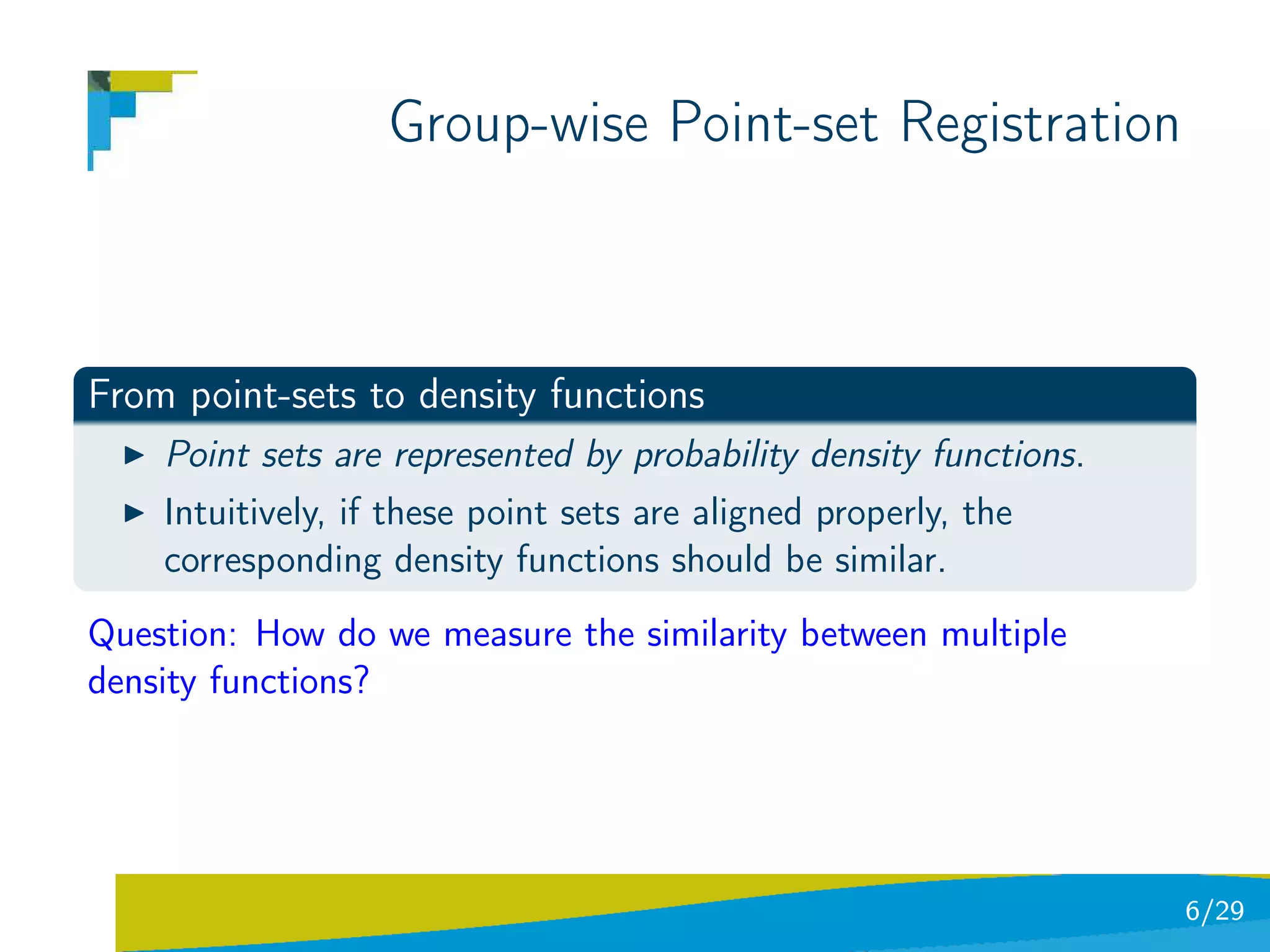
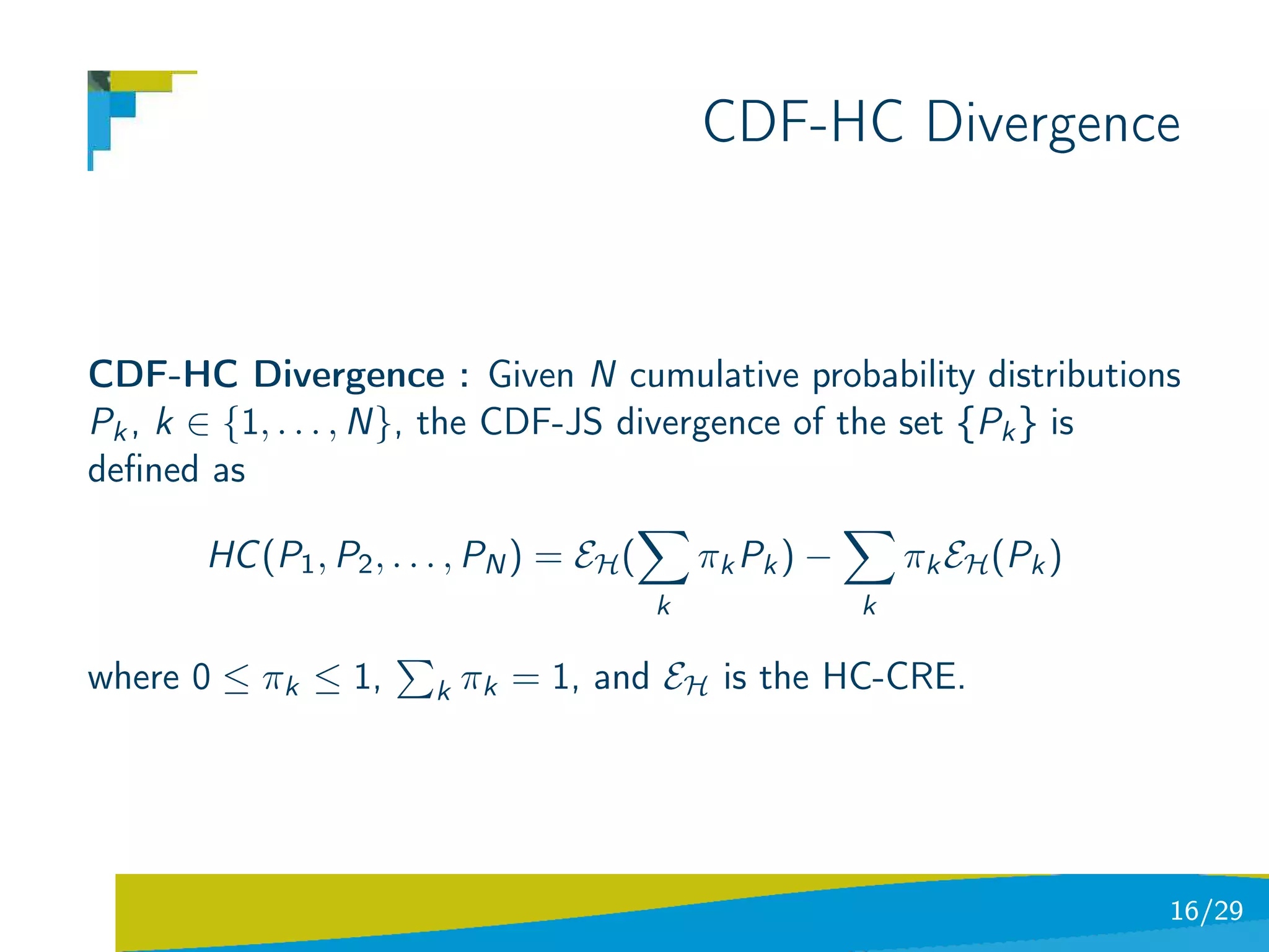
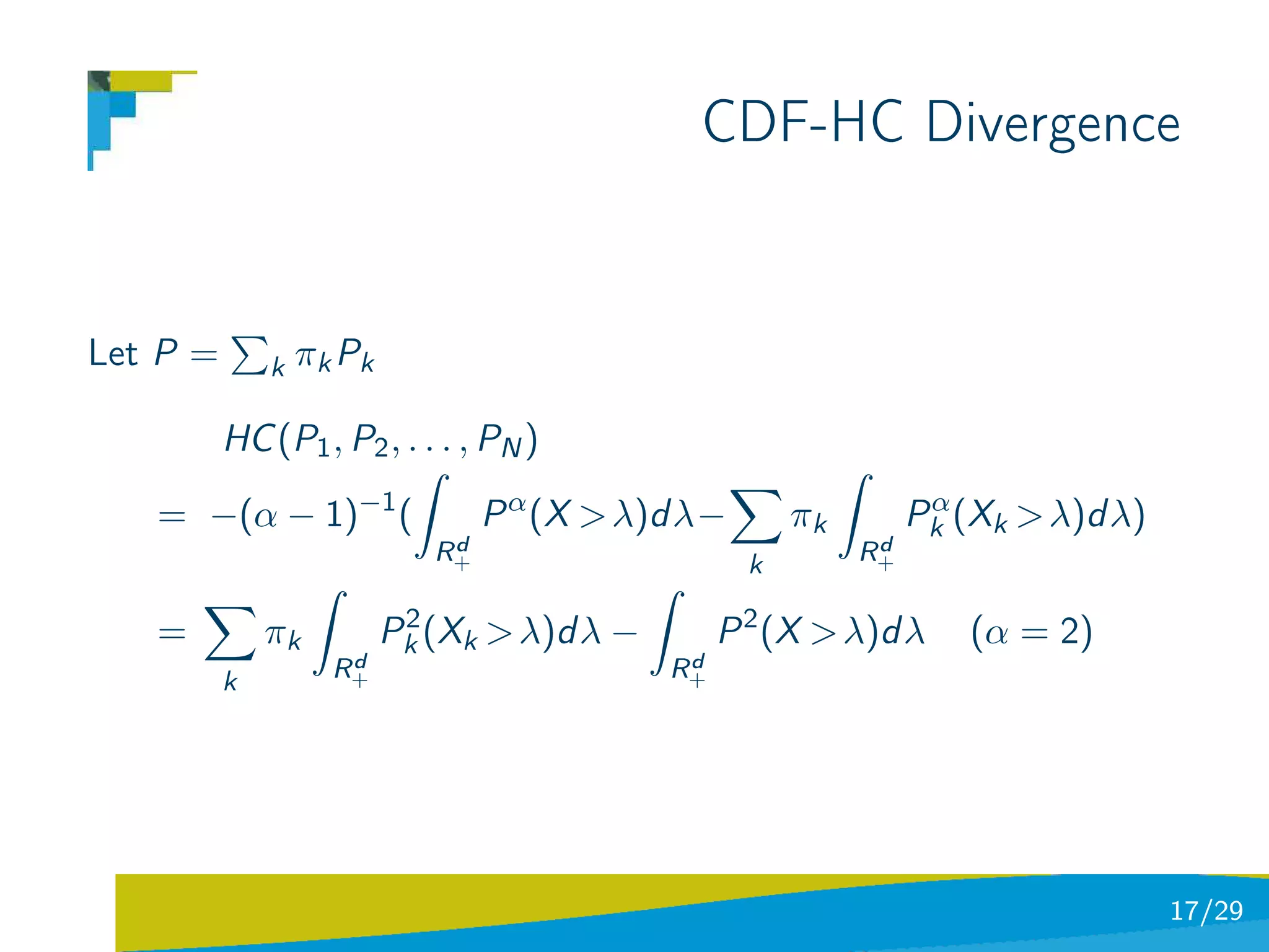
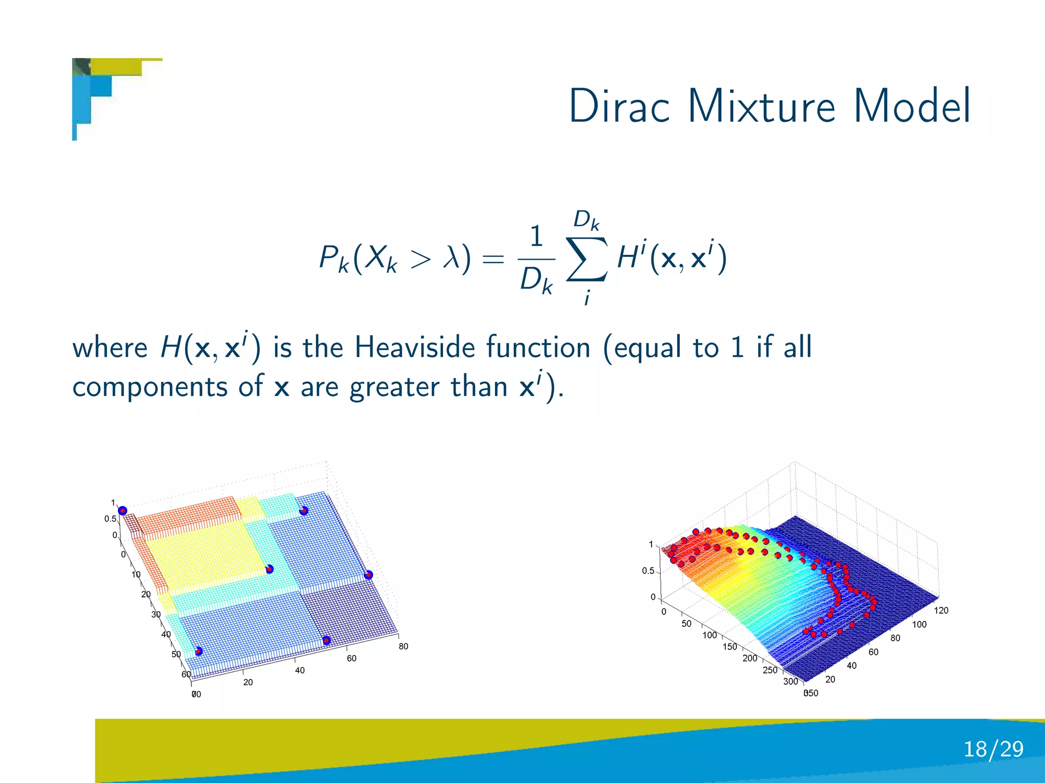
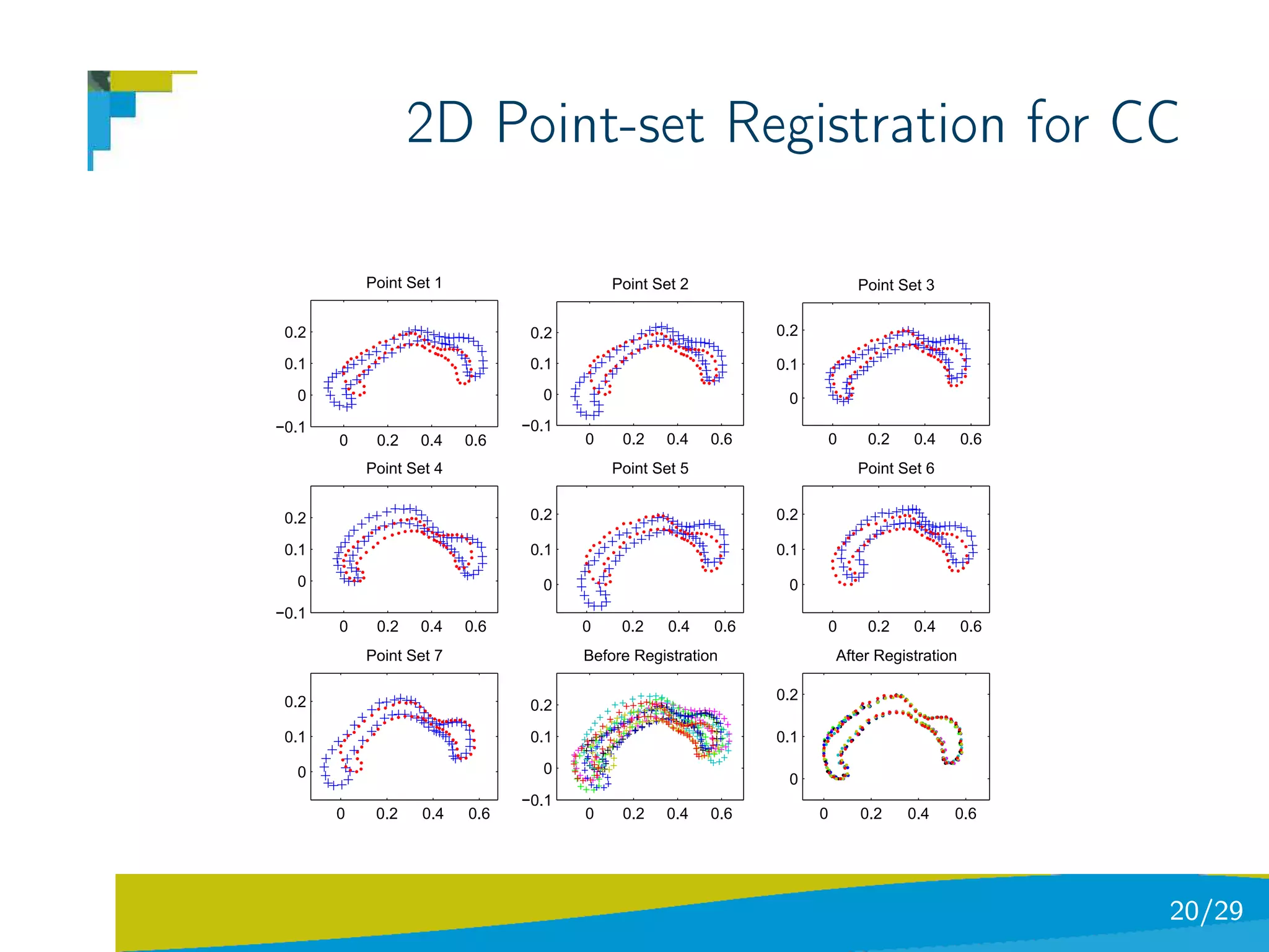
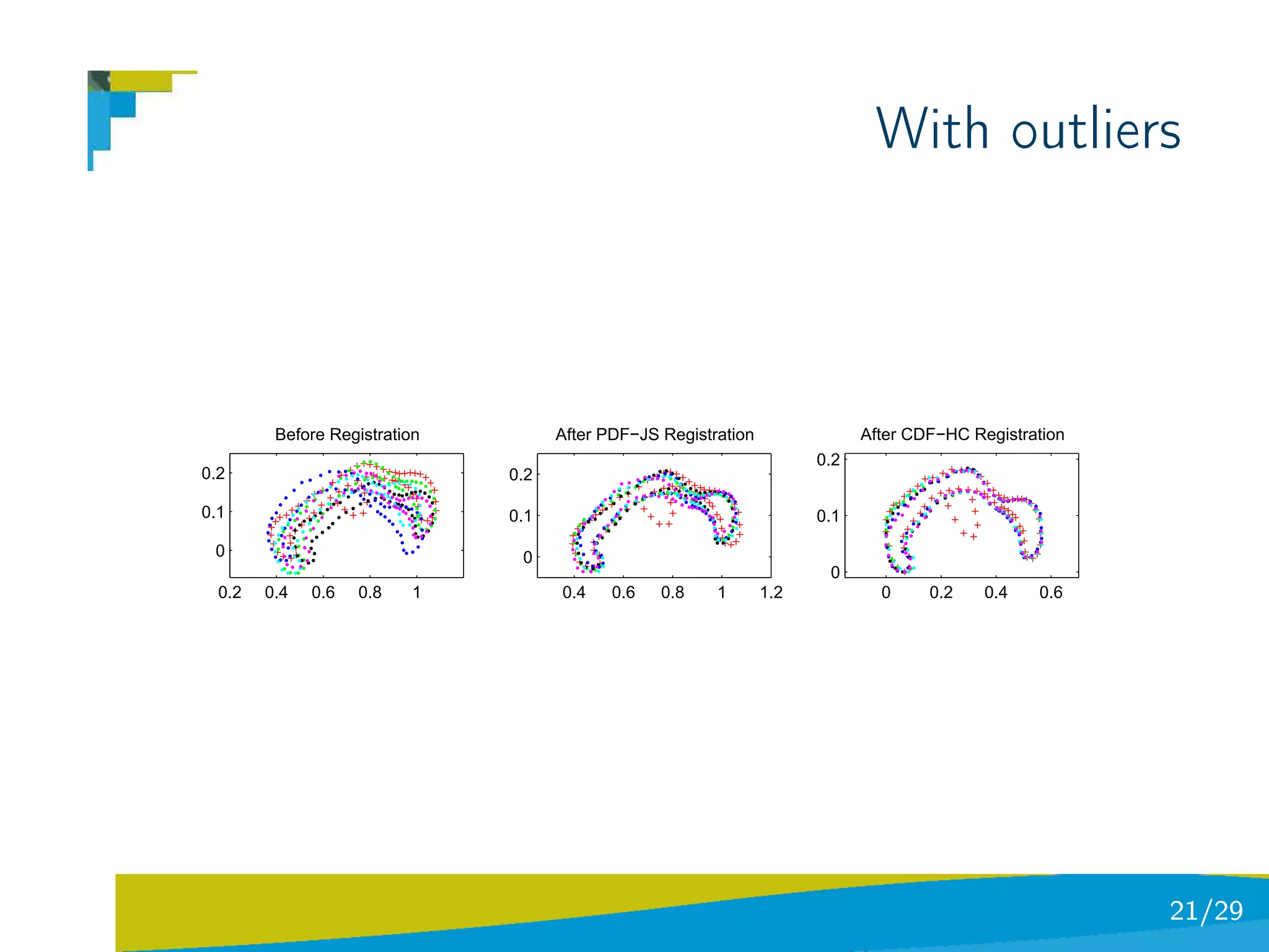
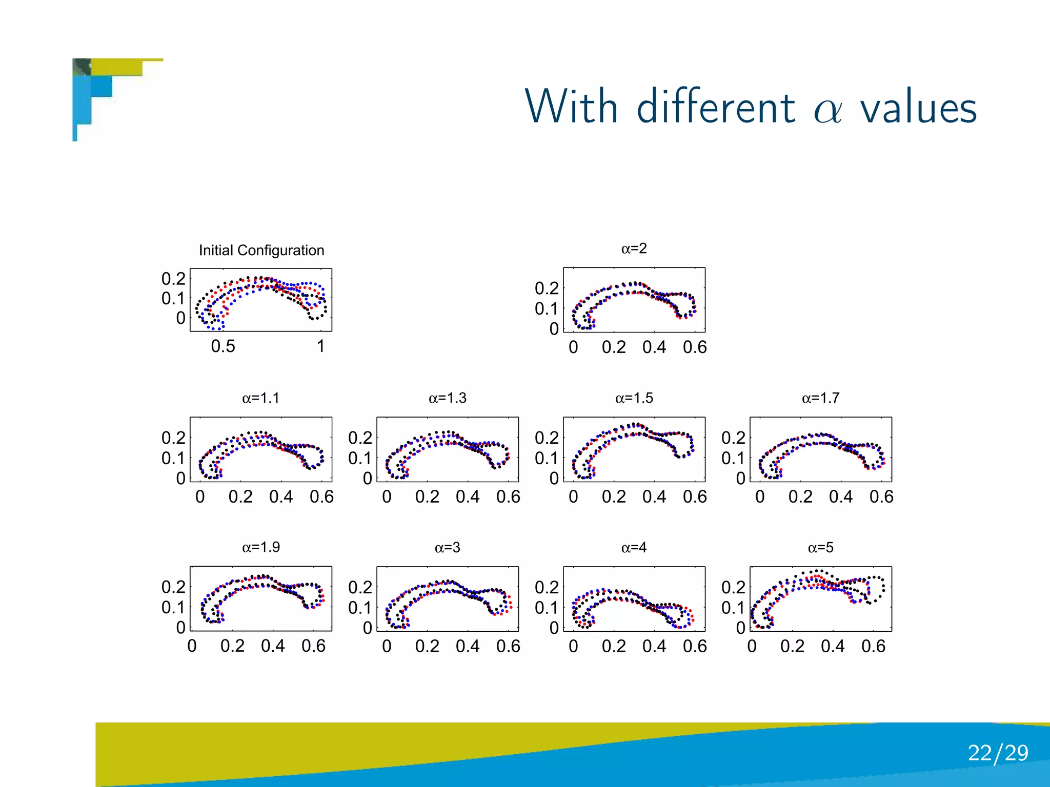
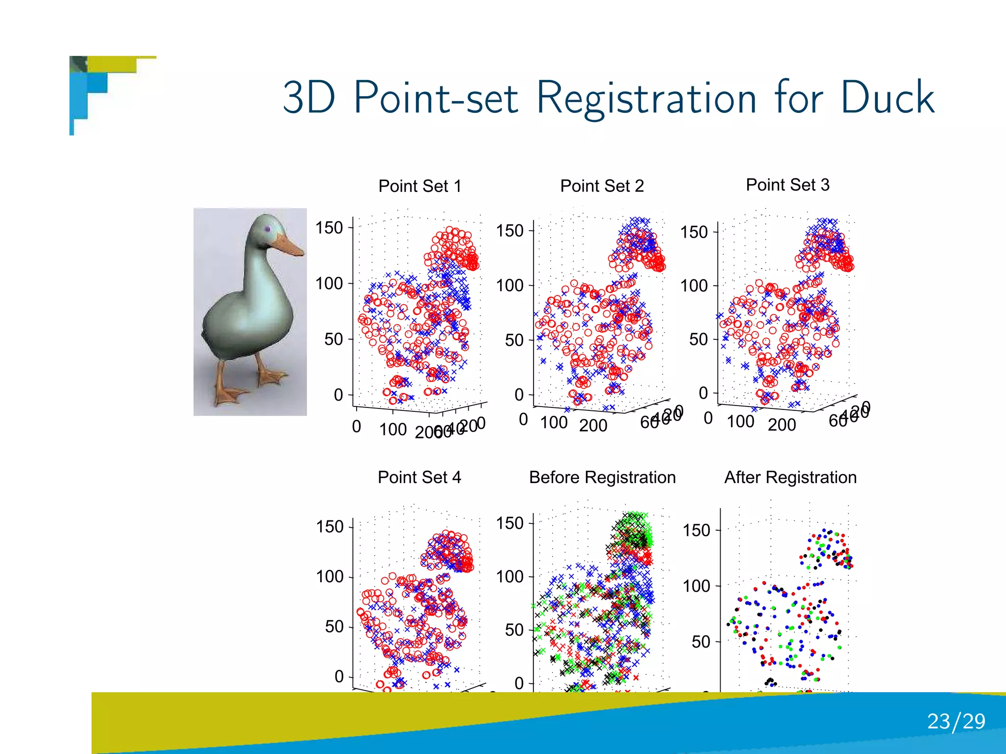
Model each point-set by a cumulative distribution function
(CDF)
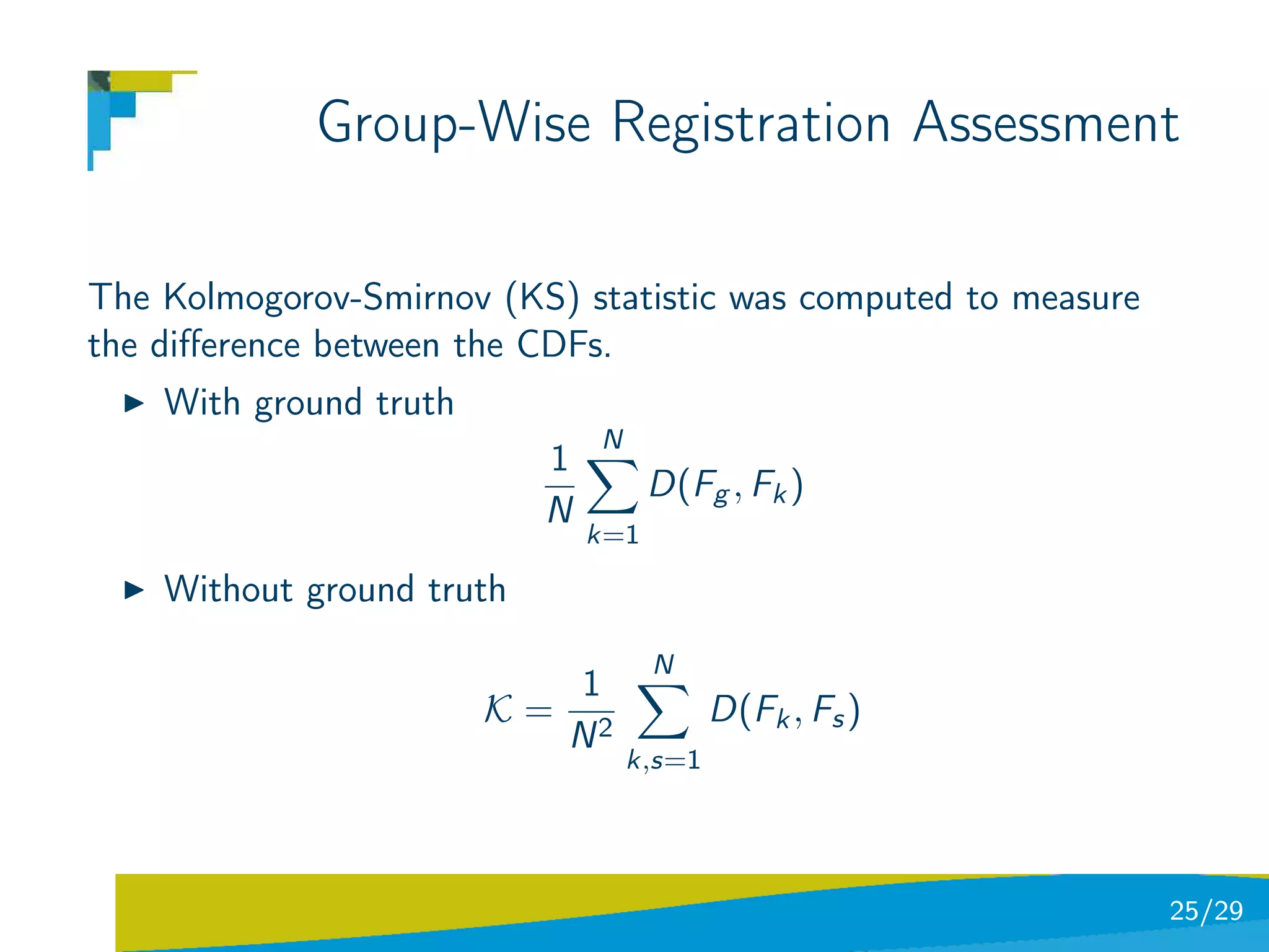
Quantify the distance among cdfs via an information-theoretic
measure [typically the cumulative residual entropy (CRE)]
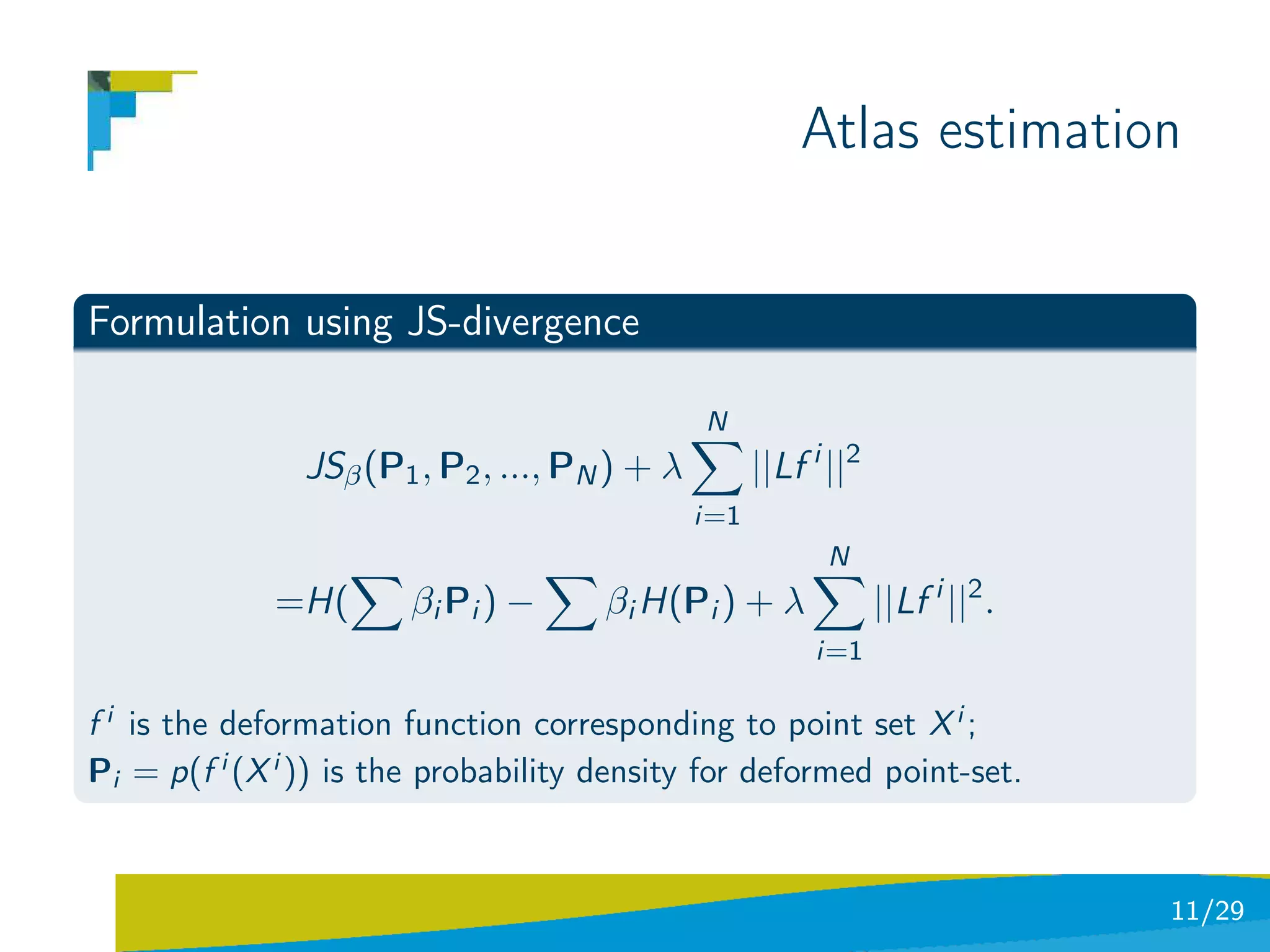
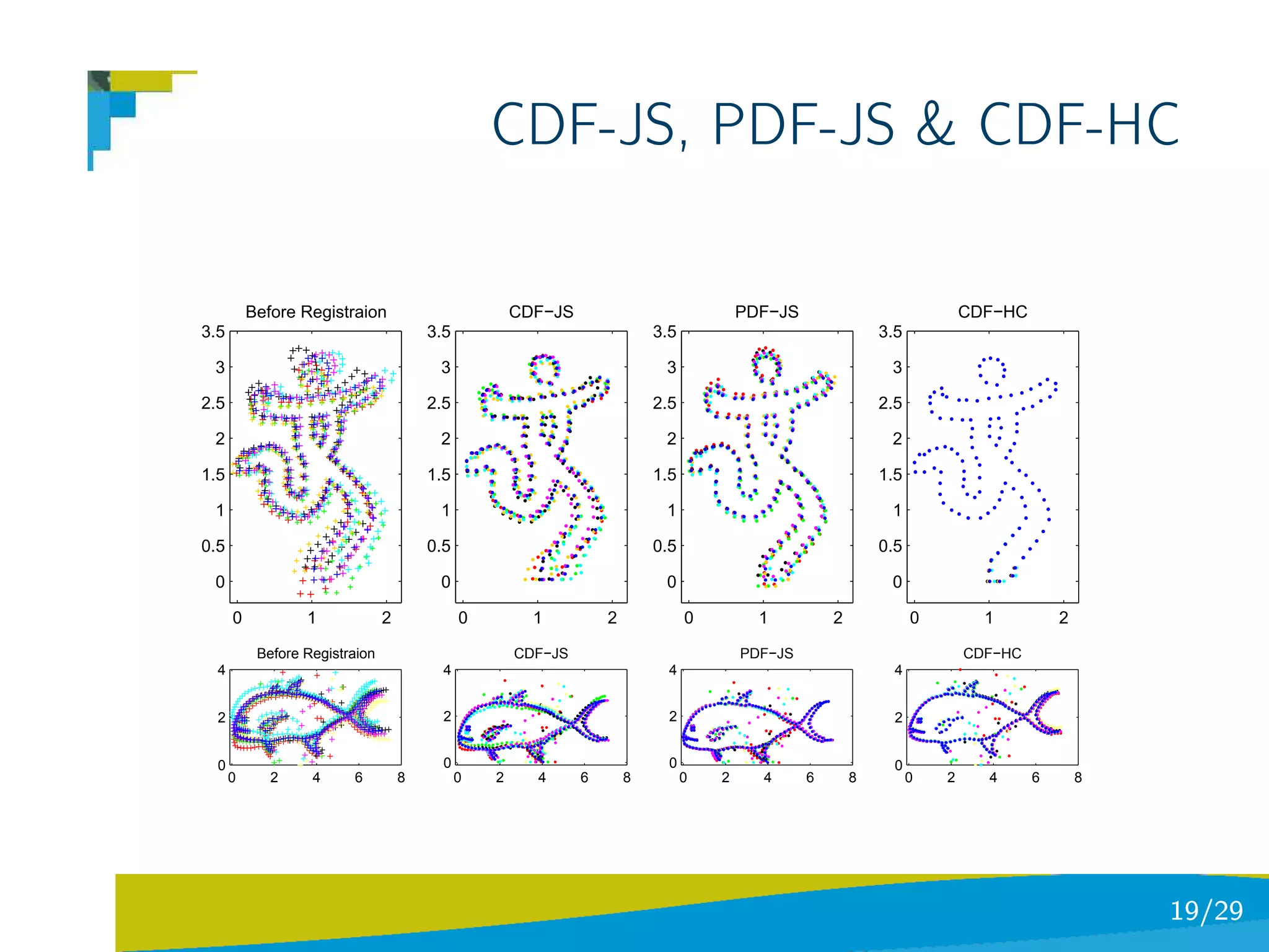
Minimize the dis-similarity measure over the space of
coordinate transformation parameters
14/29

21. Havrda-Charvát CRE
HC-CRE: Let X be a random vector in R d , we define the HC-CRE
of X by
ˆ
EH (X ) = − (α − 1)−1 (P α (|X | > λ) − P(|X | > λ))d λ
d
R+
where X = {x1 , x2 , . . . , xd }, λ = {λ1 , λ2 , . . . , λd }, and |X | > λ
means |xi | > λi , R+ = {xi ∈ R d ; xi ≥ 0; i ∈ {1, 2, . . . , d }}.
d
15/29

22. CDF-HC Divergence
CDF-HC Divergence : Given N cumulative probability distributions
Pk , k ∈ {1, . . . , N}, the CDF-JS divergence of the set {Pk } is
defined as
HC (P1 , P2 , . . . , PN ) = EH ( πk Pk ) − πk EH (Pk )
k k
where 0 ≤ πk ≤ 1, k πk = 1, and EH is the HC-CRE.
16/29

23. CDF-HC Divergence
Let P = k πk Pk
HC (P1 , P2 , . . . , PN )
ˆ ˆ
−1
= −(α − 1) ( P α (X > λ)d λ− πk α
Pk (Xk > λ)d λ)
d
R+ d
R+
k
ˆ ˆ
2
= πk Pk (Xk > λ)d λ − P 2 (X > λ)d λ (α = 2)
d
R+ d
R+
k
17/29

24. Dirac Mixture Model
Dk
1
Pk (Xk > λ) = H i (x, xi )
Dk
i
where H(x, xi ) is the Heaviside function (equal to 1 if all
components of x are greater than xi ).
1
0.5
0
0
10
20
30
40
80
50 60
60 40
20
0
70
18/29

25. CDF-JS, PDF-JS & CDF-HC
Before Registraion CDF−JS PDF−JS CDF−HC
3.5 3.5 3.5 3.5
3 3 3 3
2.5 2.5 2.5 2.5
2 2 2 2
1.5 1.5 1.5 1.5
1 1 1 1
0.5 0.5 0.5 0.5
0 0 0 0
0 1 2 0 1 2 0 1 2 0 1 2
Before Registraion CDF−JS PDF−JS CDF−HC
4 4 4 4
2 2 2 2
0 0 0 0
0 2 4 6 8 0 2 4 6 8 0 2 4 6 8 0 2 4 6 8
19/29

26. 2D Point-set Registration for CC
Point Set 1 Point Set 2 Point Set 3
0.2 0.2 0.2
0.1 0.1 0.1
0 0 0
−0.1 −0.1
0 0.2 0.4 0.6 0 0.2 0.4 0.6 0 0.2 0.4 0.6
Point Set 4 Point Set 5 Point Set 6
0.2 0.2 0.2
0.1 0.1 0.1
0 0 0
−0.1
0 0.2 0.4 0.6 0 0.2 0.4 0.6 0 0.2 0.4 0.6
Point Set 7 Before Registration After Registration
0.2 0.2
0.2
0.1 0.1 0.1
0 0
0
−0.1
0 0.2 0.4 0.6 0 0.2 0.4 0.6 0 0.2 0.4 0.6
20/29

27. With outliers
Before Registration After PDF−JS Registration After CDF−HC Registration
0.2
0.2 0.2
0.1 0.1 0.1
0 0
0
0.2 0.4 0.6 0.8 1 0.4 0.6 0.8 1 1.2 0 0.2 0.4 0.6
21/29

28. With different α values
Initial Configuration α=2
0.2
0.2
0.1
0.1
0
0
0.5 1 0 0.2 0.4 0.6
α=1.1 α=1.3 α=1.5 α=1.7
0.2 0.2 0.2 0.2
0.1 0.1 0.1 0.1
0 0 0 0
0 0.2 0.4 0.6 0 0.2 0.4 0.6 0 0.2 0.4 0.6 0 0.2 0.4 0.6
α=1.9 α=3 α=4 α=5
0.2 0.2 0.2 0.2
0.1 0.1 0.1 0.1
0 0 0 0
0 0.2 0.4 0.6 0 0.2 0.4 0.6 0 0.2 0.4 0.6 0 0.2 0.4 0.6
22/29

29. 3D Point-set Registration for Duck
Point Set 1 Point Set 2 Point Set 3
150 150 150
100 100 100
50 50 50
0 0 0
0
0 100 200 40 0 0 100 200 40 0
60 20 0 100 200 40
60
20
60 20
Point Set 4 Before Registration After Registration
150 150 150
100 100
100
50 50
50
0 0
0 0
0 100
200 604020 0 100 200 40 0
60 20 0 0
100 200 50 23/29

30. 3D Registration of Hippocampi
Point Set 1 Point Set 2 Point Set 3
100 0 100 0 100 0
100 100 100
200 200 200
0 0 0
50 50 50
10 10 10
20 20 20
0 0 0
Point Set 4 Point Sets Before Registration Point sets After Registration
100 0 100 0 100 0
100 100 100
200 50 50
50 0 200 200
0 0
10 5
10
20 0 10
0
0 15 20
24/29

31. Group-Wise Registration Assessment
The Kolmogorov-Smirnov (KS) statistic was computed to measure
the difference between the CDFs.
With ground truth
N
1
D(Fg , Fk )
N
k=1
Without ground truth
N
1
K= D(Fk , Fs )
N2
k,s=1
25/29

32. KS statistic for comparison
Table: KS statistic
KS-statistic CDF-JS PDF-JS CDF-HC
Olympic Logo 0.1103 0.1018 0.0324
Fish with outliers 0.1314 0.1267 0.0722
Table: Average nearest neighbor distance
ANN distance CDF-JS PDF-JS CDF-HC
Olympic Logo 0.0367 0.0307 0.0019
Fish with outliers 0.0970 0.0610 0.0446
26/29

33. KS statistic for comparison (contd.)
Table: Non-rigid group-wise registration assessment without ground truth
using KS statistics
Before Registration After Registration
Corpus Callosum 0.3226 0.0635
Corpus Callosum with outlier 0.3180 0.0742
Olympic Logo 0.1559 0.0308
Fish 0.1102 0.0544
Hippocampus 0.2620 0.0770
Duck 0.2287 0.0160
27/29

34. KS statistic for comparison (contd.)
Table: Non-rigid group-wise registration assessment without ground truth
using average nearest neighbor distance
Before Registration After Registration
Corpus Callosum 0.0291 0.0029
Corpus Callosum with outlier 0.0288 0.0092
Olympic Logo 0.0825 0.0022
Fish 0.1461 0.0601
Hippocampus 13.7679 3.1779
Duck 15.4725 0.3280
28/29

35. Discussion
I-divergences for shape matching avoid correspondence problem
Symmetric, unbiased registration and atlas estimation
Shape densities modeled as Gaussian mixtures, cumulatives
directly estimated
JS (pdf and cdf-based) and HC divergences used
Estimated atlas useful in model-based segmentation
29/29