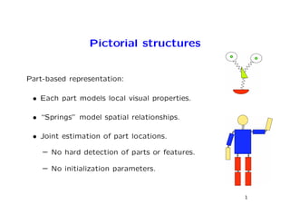
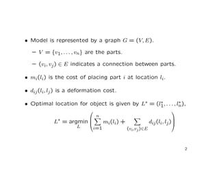
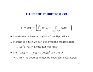
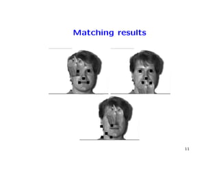
Object Recognition with Pictorial Structures

                Pedro F. Felzenszwalb
                University of Chicago
                 pff@cs.uchicago.edu

        Joint work with Daniel P. Huttenlocher
Pictorial structures


Part-based representation:

 • Each part models local visual properties.

 • “Springs” model spatial relationships.

 • Joint estimation of part locations.

    – No hard detection of parts or features.

    – No initialization parameters.


                                                1
• Model is represented by a graph G = (V, E).

   – V = {v1, . . . , vn} are the parts.

   – (vi, vj ) ∈ E indicates a connection between parts.

• mi(li) is the cost of placing part i at location li.

• dij (li, lj ) is a deformation cost.

• Optimal location for object is given by L∗ = (l1, . . . , ln),
                                                 ∗           ∗
                                                            
                          n
            L∗ = argmin     mi(li) +            dij (li, lj )
                                                              
                        
                    L    i=1          (vi,vj )∈E


                                                                  2
Efficient minimization

                                                           
                         n
          L∗ = argmin      mi(li) +            dij (li, lj )
                                                            
                  L     i=1          (vi,vj )∈E

• n parts and h locations gives hn configurations.

• If graph is a tree we can use dynamic programming.

   – O(nh2), much better but still slow.

• If dij (li, lj ) = ||Tij (li) − Tji(lj )||2 can use DT.

   – O(nh), as good as matching each part separately!!

                                                                 3
Distance transform
 Given a set of points on a grid P ⊆ G,
the quadratic distance transform of P is,


          DP (q) = min ||q − p||2
                    p∈P


           P                DP

                                            4
Generalized distance transform


Given a function f : G → R,

                 Df (q) = min ||q − p||2 + f (p)
                              p∈G

 – for each location q, find nearby location p with f (p) small.

 – equals DT of points P if f is an indicator function.
                                    
                                    0   if p ∈ P
                       f (p) =                     .
                                    ∞   otherwise


                                                           5
1D case:      Df (q) = minp∈G (q − p)2 + f (p)

For each p, Df (q) is below the parabola rooted at (p, f (p)).

Df (q) is defined by the lower envelope of h parabolas.
                                          1
                          f


                              (


                                              )
                                      2
                          f


                              (


                                              )
                                  §
                      h


                                          1
                  f


                      (


                                              )
                                      0
                          f


                              (


                                              )


                                                                                                                      §
                                                              .


                                                                  .


                                                                      .


                                                                          .


                                                                              .


                                                                                  .


                                                                                      .


                                                                                          .


                                                                                              .


                                                                                                  .


                                                                                                      .


                                                                                                          .


                                                                                                              .
                                                  0


                                                      1


                                                          2


                                                                                                                  h


                                                                                                                          1


                                                                                                                              6
There is a simple geometric algorithm that computes Df (p) in
O(h) time for the 1D case.

 – similar to Graham’s scan convex hull algorithm.

 – about 20 lines of C code.


The 2D case is “separable”, it can be solved by sequential 1D
transformations along rows and columns of the grid.

See Distance Transforms of Sampled Functions, Felzen-
szwalb and Huttenlocher.


                                                        7
Simple face model

• Locations are positions in the image grid.

• Match cost mi(li) for placing part i at li.

• Central part v1 - the nose.

• Each part has an ideal position pi relative to nose.

  – Let T1i(l1) = l1 + pi,

                               n                n
        E(l1, . . . , ln) =         mi(li) +         ||li − T1i(l1)||2
                              i=1              i=2


                                                                         8
Efficient minimization

                                                            
                   n                n
L∗ = argmin            mi(li) +             ||li − T1i(l1)||2
        L         i=1              i=2
                                                                 
                              n
L∗ = argmin m1(l1) +              mi(li) + ||li − T1i(l1)||2
        L                    i=2
                                                                     
                              n
 ∗
l1 = argmin m1(l1) +              min(mi(li) + ||li − T1i(l1)||2)
        l1                   i=2        li

                                                       
                              n
 ∗
l1 = argmin m1(l1) +              Dmi (T1i(l1))
        l1                   i=2
                                                                      9
Matching results


                   10
Matching results


                   11
Summary


• Generic framework for part-based modeling.


• Global minimization for deformable objects can be fast.


• Soft detection avoids unnecessary early decisions.


• Partial occlusion is handled automatically.


                                                        12

Object recognition with pictorial structures

  • 1.
    Object Recognition withPictorial Structures Pedro F. Felzenszwalb University of Chicago pff@cs.uchicago.edu Joint work with Daniel P. Huttenlocher
  • 2.
    Pictorial structures Part-based representation: • Each part models local visual properties. • “Springs” model spatial relationships. • Joint estimation of part locations. – No hard detection of parts or features. – No initialization parameters. 1
  • 3.
    • Model isrepresented by a graph G = (V, E). – V = {v1, . . . , vn} are the parts. – (vi, vj ) ∈ E indicates a connection between parts. • mi(li) is the cost of placing part i at location li. • dij (li, lj ) is a deformation cost. • Optimal location for object is given by L∗ = (l1, . . . , ln), ∗ ∗   n L∗ = argmin  mi(li) + dij (li, lj )   L i=1 (vi,vj )∈E 2
  • 4.
    Efficient minimization   n L∗ = argmin  mi(li) + dij (li, lj )   L i=1 (vi,vj )∈E • n parts and h locations gives hn configurations. • If graph is a tree we can use dynamic programming. – O(nh2), much better but still slow. • If dij (li, lj ) = ||Tij (li) − Tji(lj )||2 can use DT. – O(nh), as good as matching each part separately!! 3
  • 5.
    Distance transform Givena set of points on a grid P ⊆ G, the quadratic distance transform of P is, DP (q) = min ||q − p||2 p∈P P DP 4
  • 6.
    Generalized distance transform Givena function f : G → R, Df (q) = min ||q − p||2 + f (p) p∈G – for each location q, find nearby location p with f (p) small. – equals DT of points P if f is an indicator function.  0 if p ∈ P f (p) = . ∞ otherwise 5
  • 7.
    1D case: Df (q) = minp∈G (q − p)2 + f (p) For each p, Df (q) is below the parabola rooted at (p, f (p)). Df (q) is defined by the lower envelope of h parabolas. 1 f ( ) 2 f ( ) § h 1 f ( ) 0 f ( ) § . . . . . . . . . . . . . 0 1 2 h 1 6
  • 8.
    There is asimple geometric algorithm that computes Df (p) in O(h) time for the 1D case. – similar to Graham’s scan convex hull algorithm. – about 20 lines of C code. The 2D case is “separable”, it can be solved by sequential 1D transformations along rows and columns of the grid. See Distance Transforms of Sampled Functions, Felzen- szwalb and Huttenlocher. 7
  • 9.
    Simple face model •Locations are positions in the image grid. • Match cost mi(li) for placing part i at li. • Central part v1 - the nose. • Each part has an ideal position pi relative to nose. – Let T1i(l1) = l1 + pi, n n E(l1, . . . , ln) = mi(li) + ||li − T1i(l1)||2 i=1 i=2 8
  • 10.
    Efficient minimization   n n L∗ = argmin  mi(li) + ||li − T1i(l1)||2 L i=1 i=2   n L∗ = argmin m1(l1) + mi(li) + ||li − T1i(l1)||2 L i=2   n ∗ l1 = argmin m1(l1) + min(mi(li) + ||li − T1i(l1)||2) l1 i=2 li   n ∗ l1 = argmin m1(l1) + Dmi (T1i(l1)) l1 i=2 9
  • 11.
  • 12.
  • 13.
    Summary • Generic frameworkfor part-based modeling. • Global minimization for deformable objects can be fast. • Soft detection avoids unnecessary early decisions. • Partial occlusion is handled automatically. 12