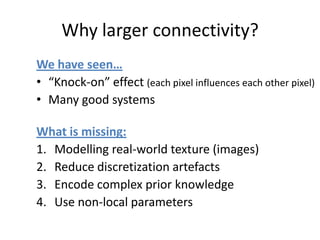
Downloaded 20 times
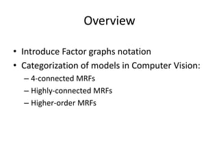


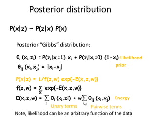
![Stereo matching - prior
θij (di,dj) = g(|di-dj|)
cost
|di-dj|
No truncation
(global min.)
[Olga Veksler PhD thesis,
Daniel Cremers et al.]](https://image.slidesharecdn.com/iccv09part2rotherdiscretemodels-1299780135-phpapp02/85/Discrete-Models-in-Computer-Vision-17-320.jpg)
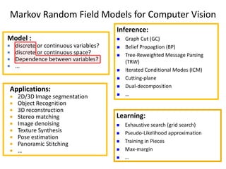
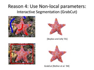
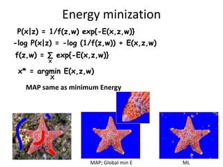
![Stereo matching - prior
θij (di,dj) = g(|di-dj|)
cost
|di-dj|
discontinuity preserving potentials
*Blake&Zisserman’83,’87+
No truncation with truncation
(global min.) (NP hard optimization)
[Olga Veksler PhD thesis,
Daniel Cremers et al.]](https://image.slidesharecdn.com/iccv09part2rotherdiscretemodels-1299780135-phpapp02/85/Discrete-Models-in-Computer-Vision-18-320.jpg)
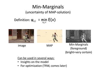
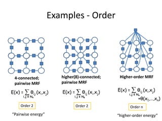
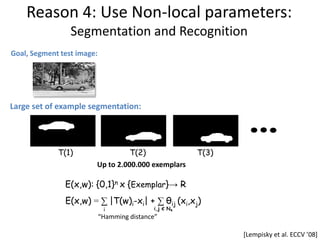
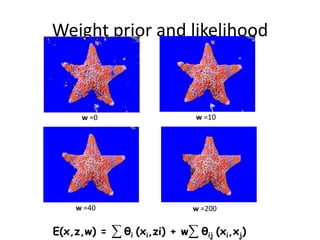
![Texture synthesis
Input
Output
Good case: Bad case:
b b b
a a
i j i j
a
E: {0,1}n → R
O E(x) = ∑ |xi-xj| [ |ai-bi|+|aj-bj| ]
i,j Є N4
1
[Kwatra et. al. Siggraph ‘03 +](https://image.slidesharecdn.com/iccv09part2rotherdiscretemodels-1299780135-phpapp02/85/Discrete-Models-in-Computer-Vision-20-320.jpg)


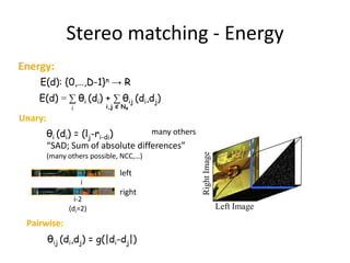
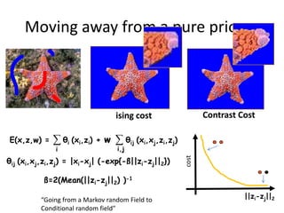
![3D reconstruction
[Slide credits: Daniel Cremers]](https://image.slidesharecdn.com/iccv09part2rotherdiscretemodels-1299780135-phpapp02/85/Discrete-Models-in-Computer-Vision-32-320.jpg)


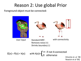
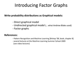
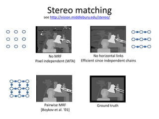
![Reason 2: Use global Prior
What is the prior of a MAP-MRF solution:
Training image: 60% black, 40% white
MAP: Others less likely :
8
prior(x) = 0.6 = 0.016 prior(x) = 0.6 5 * 0.4 3 = 0.005
MRF is a bad prior since input marginal statistic ignored !
Introduce a global term, which controls global stats:
Noisy input
Ground truth Pairwise MRF – Global gradient prior
Increase Prior strength
[Woodford et. al. ICCV ‘09]
(see poster on Friday)](https://image.slidesharecdn.com/iccv09part2rotherdiscretemodels-1299780135-phpapp02/85/Discrete-Models-in-Computer-Vision-44-320.jpg)


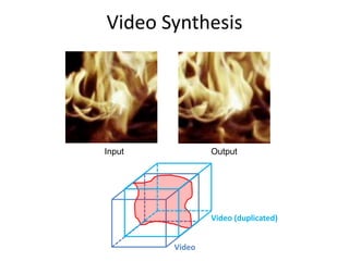
![Stereo matching - prior
θij (di,dj) = g(|di-dj|)
cost
Left image
|di-dj|
Potts model
(Potts model) Smooth disparities
[Olga Veksler PhD thesis]](https://image.slidesharecdn.com/iccv09part2rotherdiscretemodels-1299780135-phpapp02/85/Discrete-Models-in-Computer-Vision-60-320.jpg)


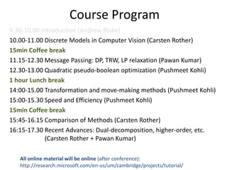
The course program includes sessions on discrete models in computer vision, message passing algorithms like dynamic programming and tree-reweighted message passing, quadratic pseudo-boolean optimization, transformation and move-making methods, speed and efficiency of algorithms, and a comparison of inference methods. Recent advances like dual decomposition and higher-order models will also be discussed. All materials from the tutorial will be made available online after the conference.