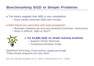
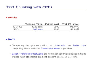
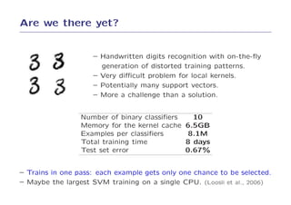
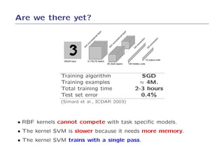
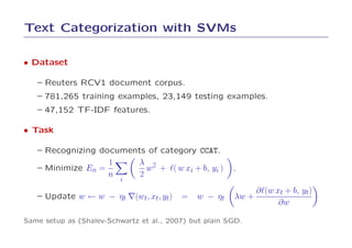
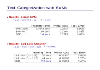
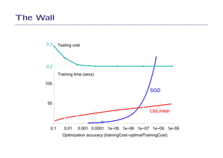
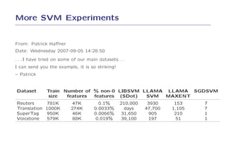
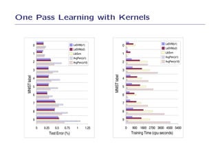
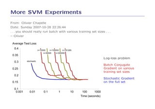
1. SGD was tested on simple learning problems like support vector machines and conditional random fields and showed competitive performance compared to specialized solvers. 2. On text categorization with SVMs, SGD achieved the same test error as SVMLight and SVMPerf but was over 100 times faster to train. 3. On log-loss classification, SGD achieved a slightly better test error than LibLinear and was over 10 times faster to train. 4. The results demonstrate that SGD can optimize simple learning problems very efficiently without the need for more complex optimization methods.

1. Learning with Large Datasets
L´on Bottou
e
NEC Laboratories America

2. Why Large-scale Datasets?
• Data Mining
Gain competitive advantages by
analyzing data that describes the life of
our computerized society.
• Artificial Intelligence
Emulate cognitive capabilities of humans.
Humans learn from abundant and diverse data.

3. The Computerized Society Metaphor
• A society with just two kinds of computers:
Makers do business and generate
← revenue. They also produce data
in proportion with their activity.
Thinkers analyze the data to
increase revenue by finding →
competitive advantages.
• When the population of computers grows:
– The ratio #Thinkers/#Makers must remain bounded.
– The Data grows with the number of Makers.
– The number of Thinkers does not grow faster than the Data.

4. Limited Computing Resources
• The computing resources available for learning
do not grow faster than the volume of data.
– The cost of data mining cannot exceed the revenues.
– Intelligent animals learn from streaming data.
• Most machine learning algorithms demand resources
that grow faster than the volume of data.
– Matrix operations (n3 time for n2 coefficients).
– Sparse matrix operations are worse.

5. Roadmap
I. Statistical Efficiency versus Computational Cost.
II. Stochastic Algorithms.
III. Learning with a Single Pass over the Examples.

6. Part I
Statistical Efficiency versus
Computational Costs.
This part is based on a joint work with Olivier Bousquet.

7. Simple Analysis
• Statistical Learning Literature:
“It is good to optimize an objective function than ensures a fast
estimation rate when the number of examples increases.”
• Optimization Literature:
“To efficiently solve large problems, it is preferable to choose
an optimization algorithm with strong asymptotic properties, e.g.
superlinear.”
• Therefore:
“To address large-scale learning problems, use a superlinear algorithm to
optimize an objective function with fast estimation rate.
Problem solved.”
The purpose of this presentation is. . .

8. Too Simple an Analysis
• Statistical Learning Literature:
“It is good to optimize an objective function than ensures a fast
estimation rate when the number of examples increases.”
• Optimization Literature:
“To efficiently solve large problems, it is preferable to choose
an optimization algorithm with strong asymptotic properties, e.g.
superlinear.”
• Therefore: (error)
“To address large-scale learning problems, use a superlinear algorithm to
optimize an objective function with fast estimation rate.
Problem solved.”
. . . to show that this is completely wrong !

9. Objectives and Essential Remarks
• Baseline large-scale learning algorithm
Randomly discarding data is the simplest
way to handle large datasets.
– What are the statistical benefits of processing more data?
– What is the computational cost of processing more data?
• We need a theory that joins Statistics and Computation!
– 1967: Vapnik’s theory does not discuss computation.
– 1981: Valiant’s learnability excludes exponential time algorithms,
but (i) polynomial time can be too slow, (ii) few actual results.
– We propose a simple analysis of approximate optimization. . .

10. Learning Algorithms: Standard Framework
• Assumption: examples are drawn independently from an unknown
probability distribution P (x, y) that represents the rules of Nature.
• Expected Risk: E(f ) = ℓ(f (x), y) dP (x, y).
1
• Empirical Risk: En(f ) = n ℓ(f (xi), yi).
• We would like f ∗ that minimizes E(f ) among all functions.
• In general f ∗ ∈ F .
/
∗
• The best we can have is fF ∈ F that minimizes E(f ) inside F .
• But P (x, y) is unknown by definition.
• Instead we compute fn ∈ F that minimizes En(f ).
Vapnik-Chervonenkis theory tells us when this can work.

11. Learning with Approximate Optimization
Computing fn = arg min En(f ) is often costly.
f ∈F
Since we already make lots of approximations,
why should we compute fn exactly?
˜
Let’s assume our optimizer returns fn
˜
such that En(fn) < En(fn) + ρ.
For instance, one could stop an iterative
optimization algorithm long before its convergence.

12. Decomposition of the Error (i)
˜
E(fn) − E(f ∗) = E(fF ) − E(f ∗)
∗ Approximation error
∗
+ E(fn) − E(fF ) Estimation error
˜
+ E(fn) − E(fn) Optimization error
Problem:
Choose F , n, and ρ to make this as small as possible,
maximal number of examples n
subject to budget constraints
maximal computing time T

13. Decomposition of the Error (ii)
Approximation error bound: (Approximation theory)
– decreases when F gets larger.
Estimation error bound: (Vapnik-Chervonenkis theory)
– decreases when n gets larger.
– increases when F gets larger.
Optimization error bound: (Vapnik-Chervonenkis theory plus tricks)
– increases with ρ.
Computing time T : (Algorithm dependent)
– decreases with ρ
– increases with n
– increases with F

14. Small-scale vs. Large-scale Learning
We can give rigorous definitions.
• Definition 1:
We have a small-scale learning problem when the active
budget constraint is the number of examples n.
• Definition 2:
We have a large-scale learning problem when the active
budget constraint is the computing time T .

15. Small-scale Learning
The active budget constraint is the number of examples.
• To reduce the estimation error, take n as large as the budget allows.
• To reduce the optimization error to zero, take ρ = 0.
• We need to adjust the size of F .
Estimation error
Approximation error
Size of F
See Structural Risk Minimization (Vapnik 74) and later works.

16. Large-scale Learning
The active budget constraint is the computing time.
• More complicated tradeoffs.
The computing time depends on the three variables: F , n, and ρ.
• Example.
If we choose ρ small, we decrease the optimization error. But we
must also decrease F and/or n with adverse effects on the estimation
and approximation errors.
• The exact tradeoff depends on the optimization algorithm.
• We can compare optimization algorithms rigorously.

17. Executive Summary
Good optimization algorithm (superlinear).
log (ρ) ρ decreases faster than exp(−T)
Mediocre optimization algorithm (linear).
ρ decreases like exp(−T)
Best ρ
Extraordinary poor
optimization algorithm
ρ decreases like 1/T
log(T)

18. Asymptotics: Estimation
Uniform convergence bounds (with capacity d + 1)
d n α 1
Estimation error ≤ O log with ≤ α ≤ 1 .
n d 2
There are in fact three types of bounds to consider:
d
– Classical V-C bounds (pessimistic): O n
d n
– Relative V-C bounds in the realizable case: O log
n d
α
d n
– Localized bounds (variance, Tsybakov): O log
n d
Fast estimation rates are a big theoretical topic these days.

19. Asymptotics: Estimation+Optimization
Uniform convergence arguments give
d n α
Estimation error + Optimization error ≤ O log + ρ .
n d
This is true for all three cases of uniform convergence bounds.
Scaling laws for ρ when F is fixed
The approximation error is constant.
α
– No need to choose ρ smaller than O d n
n log d .
α
– Not advisable to choose ρ larger than O d n
n log d .

20. . . . Approximation+Estimation+Optimization
When F is chosen via a λ-regularized cost
– Uniform convergence theory provides bounds for simple cases
(Massart-2000; Zhang 2005; Steinwart et al., 2004-2007; . . . )
– Computing time depends on both λ and ρ.
– Scaling laws for λ and ρ depend on the optimization algorithm.
When F is realistically complicated
Large datasets matter
– because one can use more features,
– because one can use richer models.
Bounds for such cases are rarely realistic enough.
Luckily there are interesting things to say for F fixed.

21. Case Study
Simple parametric setup
– F is fixed.
– Functions fw (x) linearly parametrized by w ∈ Rd.
Comparing four iterative optimization algorithms for En(f )
1. Gradient descent.
2. Second order gradient descent (Newton).
3. Stochastic gradient descent.
4. Stochastic second order gradient descent.

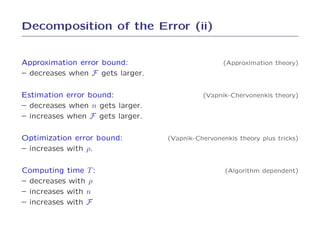
22. Quantities of Interest
• Empirical Hessian at the empirical optimum wn.
n
∂ 2En 1 ∂ 2ℓ(fn(xi), yi)
H = (fwn ) =
∂w2 n ∂w2
i=1
• Empirical Fisher Information matrix at the empirical optimum wn.
n
1 ∂ℓ(fn(xi), yi) ∂ℓ(fn(xi), yi) ′
G =
n ∂w ∂w
i=1
• Condition number
We assume that there are λmin, λmax and ν such that
– trace GH −1 ≈ ν .
– spectrum H ⊂ [λmin, λmax].
and we define the condition number κ = λmax/λmin.

23. Gradient Descent (GD)
Gradient J
Iterate
∂En(fwt )
• wt+1 ← wt − η
∂w
Best speed achieved with fixed learning rate η = λ 1 .
max
(e.g., Dennis & Schnabel, 1983)
Cost per Iterations Time to reach Time to reach
iteration to reach ρ accuracy ρ ˜ ∗
E(fn) − E(fF ) < ε
2κ
GD O(nd) 1
O κ log ρ 1
O ndκ log ρ O d1/α log2 ε
1
ε
– In the last column, n and ρ are chosen to reach ε as fast as possible.
– Solve for ε to find the best error rate achievable in a given time.
– Remark: abuses of the O() notation

24. Second Order Gradient Descent (2GD)
Gradient J
Iterate
∂En(fwt )
• wt+1 ← wt − H −1
∂w
We assume H −1 is known in advance.
Superlinear optimization speed (e.g., Dennis & Schnabel, 1983)
Cost per Iterations Time to reach Time to reach
iteration to reach ρ accuracy ρ ˜ ∗
E(fn) − E(fF ) < ε
2GD O d d+n 1
O log log ρ 1
O d d + n log log ρ O d2 log 1 log log ε
1
ε1/α ε
– Optimization speed is much faster.
– Learning speed only saves the condition number κ.

25. Stochastic Gradient Descent (SGD)
Iterate
Total Gradient <J(x,y,w)>
• Draw random example (xt, yt).
Partial Gradient J(x,y,w)
η ∂ℓ(fwt (xt), yt)
• wt+1 ← wt −
t ∂w
Best decreasing gain schedule with η = λ 1 .
min
(see Murata, 1998; Bottou & LeCun, 2004)
Cost per Iterations Time to reach Time to reach
iteration to reach ρ accuracy ρ ˜ ∗
E(fn) − E(fF ) < ε
SGD O(d) νk 1
+o ρ O dν k O dν k
ρ ρ ε
With 1 ≤ k ≤ κ2
– Optimization speed is catastrophic.
– Learning speed does not depend on the statistical estimation rate α.
– Learning speed depends on condition number κ but scales very well.

26. Second order Stochastic Descent (2SGD)
Iterate
Total Gradient <J(x,y,w)>
• Draw random example (xt, yt).
Partial Gradient J(x,y,w)
1 −1 ∂ℓ(fwt (xt), yt)
• wt+1 ← wt − H
t ∂w
η 1 −1
Replace scalar gain by matrix H .
t t
Cost per Iterations Time to reach Time to reach
iteration to reach ρ accuracy ρ ˜ ∗
E(fn) − E(fF ) < ε
2SGD O d2 ν +o 1 O d2 ν O d2 ν
ρ ρ ρ ε
– Each iteration is d times more expensive.
– The number of iterations is reduced by κ2 (or less.)
– Second order only changes the constant factors.

27. Part II
Learning with Stochastic
Gradient Descent.

28. Benchmarking SGD in Simple Problems
• The theory suggests that SGD is very competitive.
– Many people associate SGD with trouble.
• SGD historically associated with back-propagation.
– Multilayer networks are very hard problems (nonlinear, nonconvex)
– What is difficult, SGD or MLP?
• Try PLAIN SGD on simple learning problems.
– Support Vector Machines
– Conditional Random Fields
Download from http://leon.bottou.org/projects/sgd.
These simple programs are very short.
See also (Shalev-Schwartz et al., 2007; Vishwanathan et al., 2006)

29. Text Categorization with SVMs
• Dataset
– Reuters RCV1 document corpus.
– 781,265 training examples, 23,149 testing examples.
– 47,152 TF-IDF features.
• Task
– Recognizing documents of category CCAT.
1 λ 2
– Minimize En = w + ℓ( w xi + b, yi ) .
n 2
i
∂ℓ(w xt + b, yt)
– Update w ← w − ηt ∇(wt, xt, yt) = w − ηt λw +
∂w
Same setup as (Shalev-Schwartz et al., 2007) but plain SGD.

30. Text Categorization with SVMs
• Results: Linear SVM
ℓ(ˆ, y) = max{0, 1 − y y }
y ˆ λ = 0.0001
Training Time Primal cost Test Error
SVMLight 23,642 secs 0.2275 6.02%
SVMPerf 66 secs 0.2278 6.03%
SGD 1.4 secs 0.2275 6.02%
• Results: Log-Loss Classifier
ℓ(ˆ, y) = log(1 + exp(−y y )) λ = 0.00001
y ˆ
Training Time Primal cost Test Error
LibLinear (ε = 0.01) 30 secs 0.18907 5.68%
LibLinear (ε = 0.001) 44 secs 0.18890 5.70%
SGD 2.3 secs 0.18893 5.66%

31. The Wall
0.3 Testing cost
0.2
Training time (secs)
100
SGD
50
LibLinear
0.1 0.01 0.001 0.0001 1e−05 1e−06 1e−07 1e−08 1e−09
Optimization accuracy (trainingCost−optimalTrainingCost)

32. More SVM Experiments
From: Patrick Haffner
Date: Wednesday 2007-09-05 14:28:50
. . . I have tried on some of our main datasets. . .
I can send you the example, it is so striking!
– Patrick
Dataset Train Number of % non-0 LIBSVM LLAMA LLAMA SGDSVM
size features features (SDot) SVM MAXENT
Reuters 781K 47K 0.1% 210,000 3930 153 7
Translation 1000K 274K 0.0033% days 47,700 1,105 7
SuperTag 950K 46K 0.0066% 31,650 905 210 1
Voicetone 579K 88K 0.019% 39,100 197 51 1

33. More SVM Experiments
From: Olivier Chapelle
Date: Sunday 2007-10-28 22:26:44
. . . you should really run batch with various training set sizes . . .
– Olivier
Average Test Loss
0.4
n=10000 n=100000 n=781265
n=30000 n=300000
0.35
Log-loss problem
0.3 stochastic
Batch Conjugate
0.25 Gradient on various
training set sizes
0.2
Stochastic Gradient
0.15 on the full set
0.1
0.001 0.01 0.1 1 10 100 1000
Time (seconds)

34. Text Chunking with CRFs
• Dataset
– CONLL 2000 Chunking Task:
Segment sentences in syntactically correlated chunks
(e.g., noun phrases, verb phrases.)
– 106,978 training segments in 8936 sentences.
– 23,852 testing segments in 2012 sentences.
• Model
– Conditional Random Field (all linear, log-loss.)
– Features are n-grams of words and part-of-speech tags.
– 1,679,700 parameters.
Same setup as (Vishwanathan et al., 2006) but plain SGD.

35. Text Chunking with CRFs
• Results
Training Time Primal cost Test F1 score
L-BFGS 4335 secs 9042 93.74%
SGD 568 secs 9098 93.75%
• Notes
– Computing the gradients with the chain rule runs faster than
computing them with the forward-backward algorithm.
– Graph Transformer Networks are nonlinear conditional random fields
trained with stochastic gradient descent (Bottou et al., 1997).

36. Choosing the Gain Schedule
η
Decreasing gains: wt+1 ← wt − ∇(wt, xt, yt)
t + t0
• Asymptotic Theory
– if s = 2 η λmin < 1 then slow rate O t−s
s2
– if s = 2 η λmin > 1 then faster rate O s−1 t−1
• Example: the SVM benchmark
– Use η = 1/λ because λ ≤ λmin.
– Choose t0 to make sure that the expected initial updates
are comparable with the expected size of the weights.
• Example: the CRF benchmark
– Use η = 1/λ again.
– Choose t0 with the secret ingredient.

37. The Secret Ingredient for a good SGD
The sample size n does not change the SGD maths!
Constant gain: wt+1 ← wt − η ∇(wt, xt, yt)
At any moment during training, we can:
– Select a small subsample of examples.
– Try various gains η on the subsample.
– Pick the gain η that most reduces the cost.
– Use it for the next 100000 iterations on the full dataset.
• Examples
– The CRF benchmark code does this to choose t0 before training.
– We could also perform such cheap measurements every so often.
The selected gains would then decrease automatically.

38. Getting the Engineering Right
The very simple SGD update offers lots of engineering opportunities.
Example: Sparse Linear SVM
The update w ← w − η λw − ∇ℓ(wxi, yi)
can be performed in two steps:
i) w ← w − η∇ℓ(wxi, yi) (sparse, cheap)
ii) w ← w (1 − ηλ) (not sparse, costly)
• Solution 1
Represent vector w as the product of a scalar s and a vector v .
Perform (i) by updating v and (ii) by updating s.
• Solution 2
Perform only step (i) for each training example.
Perform step (ii) with lower frequency and higher gain.

39. SGD for Kernel Machines
• SGD for Linear SVM
– Both w and ∇ℓ(wxt, yt) represented using coordinates.
– SGD updates w by combining coordinates.
• SGD for SVM with Kernel K(xi, xj ) = < Φ(xi), Φ(xj ) >
– Represent w with its kernel expansion αi Φ(xi).
– Usually, ∇ℓ(wxt, yt) = −µ Φ(xt).
– SGD updates w by combining coefficients:
η µ if i = t,
αi ←− (1 − ηλ) αi +
0 otherwise.
• So, one just needs a good sparse vector library ?

40. SGD for Kernel Machines
• Sparsity Problems.
η µ if i = t,
αi ←− (1 − ηλ) αi +
0 otherwise.
– Each iteration potentially makes one α coefficient non zero.
– Not all of them should be support vectors.
– Their α coefficients take a long time to reach zero (Collobert, 2004).
• Dual algorihms related to primal SGD avoid this issue.
– Greedy algorithms (Vincent et al., 2000; Keerthi et al., 2007)
– LaSVM and related algorithms (Bordes et al., 2005)
More on them later. . .
• But they still need to compute the kernel values!
– Computing kernel values can be slow.
– Caching kernel values can require lots of memory.

41. SGD for Real Life Applications
A Check Reader
Examples are pairs (image,amount).
Problem with strong structure:
– Field segmentation
– Character segmentation
– Character recognition
– Syntactical interpretation.
• Define differentiable modules.
• Pretrain modules with hand-labelled data.
• Define global cost function (e.g., CRF).
• Train with SGD for a few weeks.
Industrially deployed in 1996. Ran billions of checks over 10 years.
Credits: Bengio, Bottou, Burges, Haffner, LeCun, Nohl, Simard, et al.

42. Part III
Learning with a Single Pass
over the Examples
This part is based on joint works with
Antoine Bordes, Seyda Ertekin, Yann LeCun, and Jason Weston.

43. Why learning with a Single Pass?
• Motivation
– Sometimes there is too much data to store.
– Sometimes retrieving archived data is too expensive.
• Related Topics
– Streaming data.
– Tracking nonstationarities.
– Novelty detection.
• Outline
– One-pass learning with second order SGD.
– One-pass learning with kernel machines.
– Comparisons

44. Effect of one Additional Example (i)
Compare
∗
wn = arg min En(fw )
w
∗ 1
wn+1 = arg min En+1(fw ) = arg min En(fw ) + ℓ fw (xn+1), yn+1
w w n
n+1
E (f )
n n+1 w
En(f w )
w*
n+1 w*
n

45. Effect of one Additional Example (ii)
• First Order Calculation
∗ ∗ 1 −1 ∂ ℓ fwn (xn), yn 1
wn+1 = wn − Hn+1 + O
n ∂w n2
where Hn+1 is the empirical Hessian on n + 1 examples.
• Compare with Second Order Stochastic Gradient Descent
1 ∂ ℓ fwt (xn), yn
wt+1 = wt − H −1
t ∂w
• Could they converge with the same speed?

46. Yes they do! But what does it mean?
• Theorem (Bottou & LeCun, 2003; Murata & Amari, 1998)
Under “adequate conditions”
lim ∗ ∗
n w∞ − wn 2 = lim t w∞ − wt 2 = tr(H −1G H −1)
n→∞ t→∞
lim n E(fwn ) − E(fF ) = lim t E(fwt ) − E(fF ) = tr(G H −1)
∗
n→∞ t→∞
Best solution in F.
One Pass of w∞=w*
∞
Second Order
Stochastic
w
Gradient n
≅ K/n
w0= w* Empirical Best training
0
Optima w* set error.
n

47. Optimal Learning in One Pass
Given a large enough training set,
a Single Pass of Second Order Stochastic Gradient
generalizes as well as the Empirical Optimum.
Experiments on synthetic data
Mse*
+1e−1
0.366
Mse*
+1e−2 0.362
0.358
Mse*
+1e−3 0.354
Mse* 0.350
+1e−4
0.346
0.342
1000 10000 100000 100 1000 10000
Number of examples Milliseconds

48. Unfortunate Practical Issues
• Second Order SGD is not that fast!
1 ∂ℓ(fwt (xt), yt)
wt+1 ← wt − H −1
t ∂w
– Must estimate and store d × d matrix H −1.
– Must multiply the gradient for each example by the matrix H −1.
– Sparsity tricks no longer work because H −1 is not sparse.
• Research Directions
Limited storage approximations of H −1.
– Reduce the number of epochs
– Rarely sufficient for fast one-pass learning.
– Diagonal approximation (Becker &LeCun, 1989)
– Low rank approximation (e.g., LeCun et al., 1998)
– Online L-BFGS approximation (Schraudolph, 2007)

49. Disgression: Stopping Criteria for SGD
2SGD SGD
ν 1 kν 1
Time to reach accuracy ρ +o +o
ρ ρ ρ ρ
Number of epochs to reach
same test cost as the full 1 k
optimization. 1 ≤ k ≤ κ2
There are many ways to make constant k smaller:
– Exact second order stochastic gradient descent.
– Approximate second order stochastic gradient descent.
– Simple preconditionning tricks.

50. Disgression: Stopping Criteria for SGD
• Early stopping with cross validation
– Create a validation set by setting some training examples apart.
– Monitor cost function on the validation set.
– Stop when it stops decreasing.
• Early stopping a priori
– Extract two disjoint subsamples of training data.
– Train on the first subsample; stop by validating on the second.
– The number of epochs is an estimate of k.
– Train by performing that number of epochs on the full set.
This is asymptotically correct and gives reasonable results in practice.

51. One-pass learning for Kernel Machines?
Challenges for Large-Scale Kernel Machines:
– Bulky kernel matrix (n × n.)
– Managing the kernel expansion w = αi Φ(xi).
– Managing memory.
Issues of SGD for Kernel Machines:
– Conceptually simple.
– Sparsity issues in kernel expansion.
Stochastic and Incremental SVMs:
– Iteratively constructing the kernel expansion.
– Which candidate support vectors to store and discard?
– Managing the memory required by the kernel values.
– One-pass learning?

52. Learning in the dual
• Convex, Kernel trick.
• Memory n nsv
Max margin
• Time nαnsv with 1 < α ≤ 2
• Bad news nsv ∼ 2Bn
(see Steinwart, 2004)
A • nsv could be much smaller.
(Burges, 1993; Vincent & Bengio, 2002)
B Min distance
between hulls
• How to do it fast?
• How small?

53. An Inefficient Dual Optimizer
N
P
N’
• Both P and N are linear combinations of examples
with positive coefficients summing to one.
• Projection: N ′ = (1 − γ)N + γ x with 0 ≤ γ ≤ 1.
• Projection time proportional to nsv .

54. Two Problems with this Algorithm
• Eliminating unwanted Support Vectors
γ = − α / (1−α) Pattern x already has α > 0.
But we found better support vectors.
γ=0
– Simple algo decreases α too slowly.
– Same problem as SGD in fact.
– Solution: Allow γ to be slightly negative.
γ=1
• Processing Support Vectors often enough
When drawing examples randomly,
– Most have α = 0 and should remain so.
– Support vectors (α > 0) need adjustments but are rarely processed.
– Solution: Draw support vectors more often.

55. The Huller and its Derivatives
• The Huller
Repeat
PROCESS: Pick a random fresh example and project.
REPROCESS: Pick a random support vector and project.
– Compare with incremental learning and retraining.
– PROCESS potentially adds support vectors.
– REPROCESS potentially discard support vectors.
• Derivatives of the Huller
– LASVM handles soft-margins and is connected to SMO.
– LARANK handles multiclass problems and structured outputs.
(Bordes et al., 2005, 2006, 2007)

56. One Pass Learning with Kernels

57. SGD
ndk
d
0
)
(
'
comparisons: n ≫ s ≫ r and r ≈ d
S
5
&
F
4
%
a c
$
$
3
2
#
"
"
S
2SGD
6
! 1
n d2
d2
S
U
¨
C
A
C
£
E
A A
C
B B B B
S
E
A A A A
T
G
¨
@ @ @ @ @ @ @ @ @ @
9 9 9 9 9
LaSVM
8 8 8 8 8
`
7 7 7 7 7
¢
S
F
ns
D
r2
X
©
S
6
¤
T
£
¦
¢
£
S
¡
U
F
Time and Memory
¢
LibSVM
G
©
¨
ns
nr
S
T
§
£
F
¦
Careless
¥
S
Y
¤
£
F
P
G
¤
£
¢
Memory
¡
R
I
W V H
b
G
Time
G
G
6 D F
Q

58. Are we there yet?
– Handwritten digits recognition with on-the-fly
generation of distorted training patterns.
– Very difficult problem for local kernels.
– Potentially many support vectors.
– More a challenge than a solution.
Number of binary classifiers 10
Memory for the kernel cache 6.5GB
Examples per classifiers 8.1M
Total training time 8 days
Test set error 0.67%
– Trains in one pass: each example gets only one chance to be selected.
– Maybe the largest SVM training on a single CPU. (Loosli et al., 2006)

59. Are we there yet?
er
er
ay
ay
ll
ll
na
na
io
io
n
n
ut
ut
io
io
ol
ol
ct
ct
nv
nv
ne
ne
co
co
on
on
5
5
lc
lc
5x
5x
l
l
fu
fu
10 output units
29x29 input 5 (15x15) layers
50 (5x5) layers 100 hidden units
Training algorithm SGD
Training examples ≈ 4M.
Total training time 2-3 hours
Test set error 0.4%
(Simard et al., ICDAR 2003)
• RBF kernels cannot compete with task specific models.
• The kernel SVM is slower because it needs more memory.
• The kernel SVM trains with a single pass.

60. Conclusion
• Connection between Statistics and Computation.
• Qualitatively different tradeoffs for small– and large–scale.
• Plain SGD rocks in theory and in practice.
• One-pass learning feasible with 2SGD or dual techniques.
Current algorithms still slower than plain SGD.
• Important topics not addressed today:
Example selection, data quality, weak supervision.