Download as PDF, PPTX
![Other motivating examples
Brain Imaging: Model an unknown number of spatial
activation patterns in fMRI images [Kim and Smyth, NIPS
2006]
Topic Modeling: Model an unknown number of topics
across several corpora of documents [Teh et al. 2006]
…
6](https://image.slidesharecdn.com/dptutorial-1304430760-phpapp01/75/Gentle-Introduction-to-Dirichlet-Processes-6-2048.jpg)
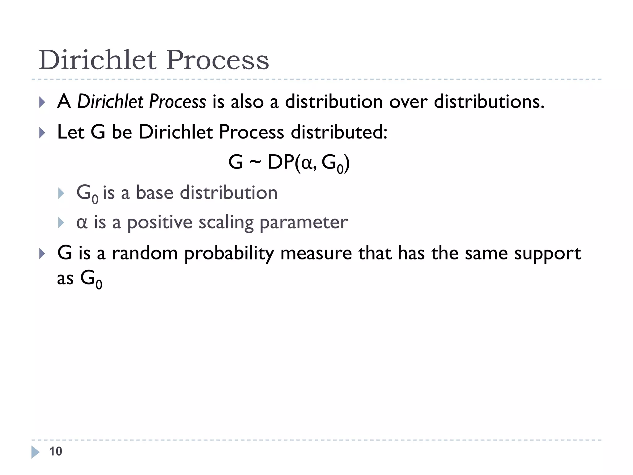
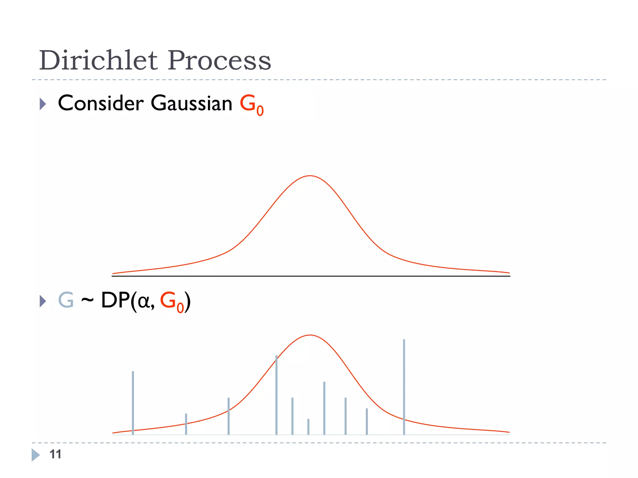
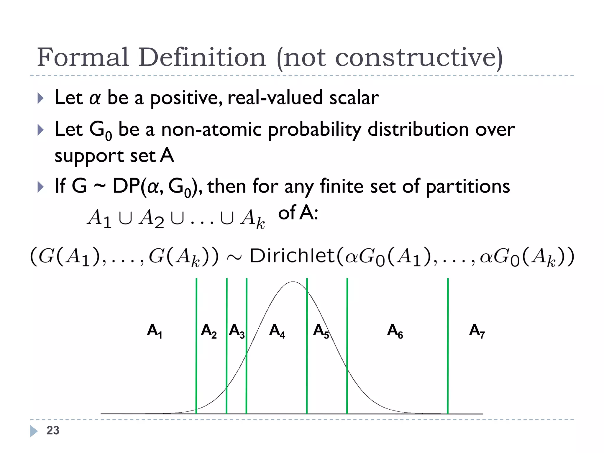
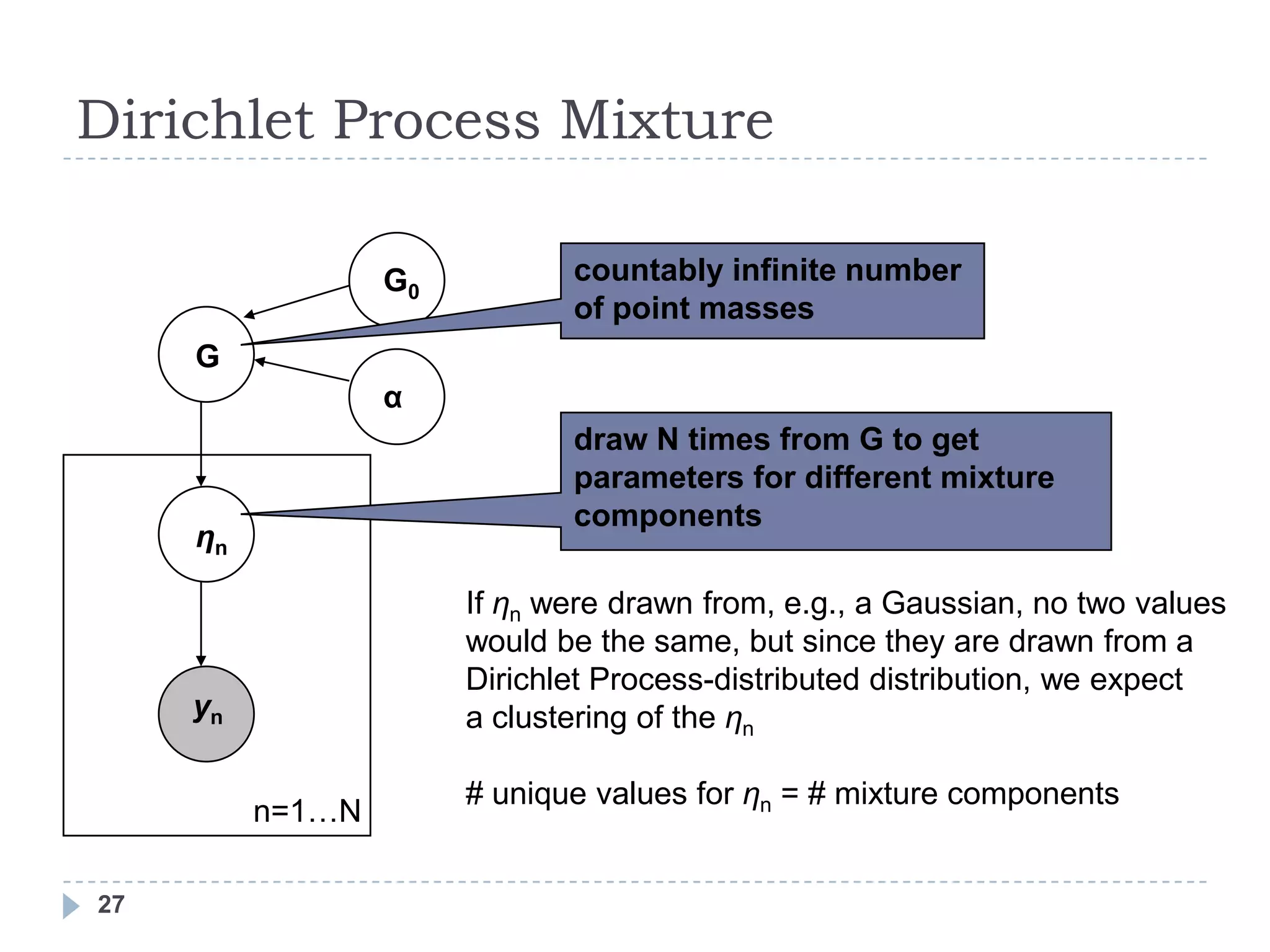
![Dirichlet Process
G ~ DP(α, G0)
G0 is continuous, so the probability that any two samples are
equal is precisely zero.
However, G is a discrete distribution, made up of a countably
infinite number of point masses [Blackwell]
Therefore, there is always a non-zero probability of two samples colliding
12](https://image.slidesharecdn.com/dptutorial-1304430760-phpapp01/75/Gentle-Introduction-to-Dirichlet-Processes-12-2048.jpg)
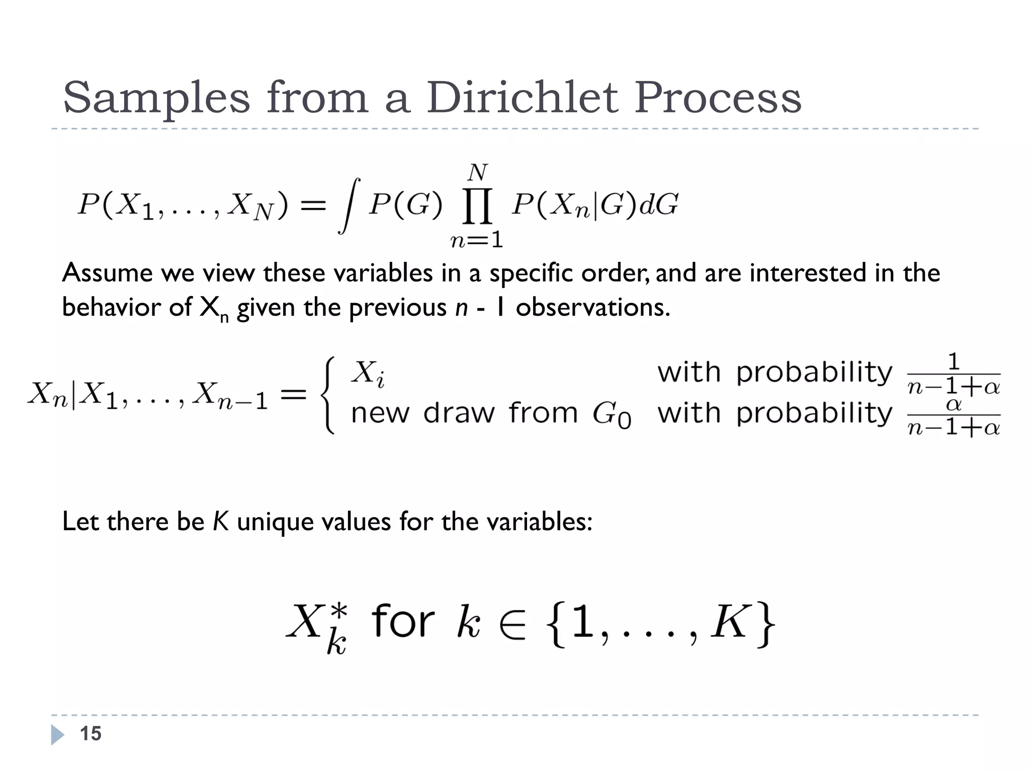
![Blackwell-MacQueen Urn Scheme
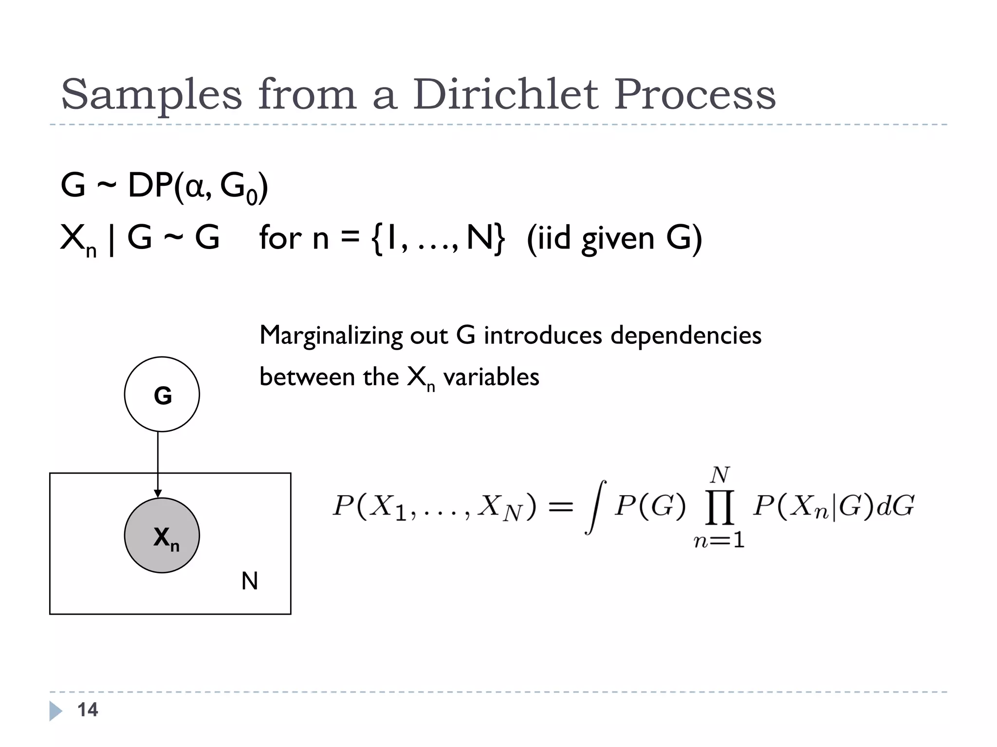
G ~ DP(α, G0)
Xn | G ~ G
Assume that G0 is a distribution over colors, and that each Xn
represents the color of a single ball placed in the urn.
Start with an empty urn.
On step n:
With probability proportional to α, draw Xn ~ G0, and add a ball of
that color to the urn.
With probability proportional to n – 1 (i.e., the number of balls
currently in the urn), pick a ball at random from the urn. Record its
color as Xn, and return the ball into the urn, along with a new one of
the same color.
[Blackwell and Macqueen, 1973]
18](https://image.slidesharecdn.com/dptutorial-1304430760-phpapp01/75/Gentle-Introduction-to-Dirichlet-Processes-18-2048.jpg)
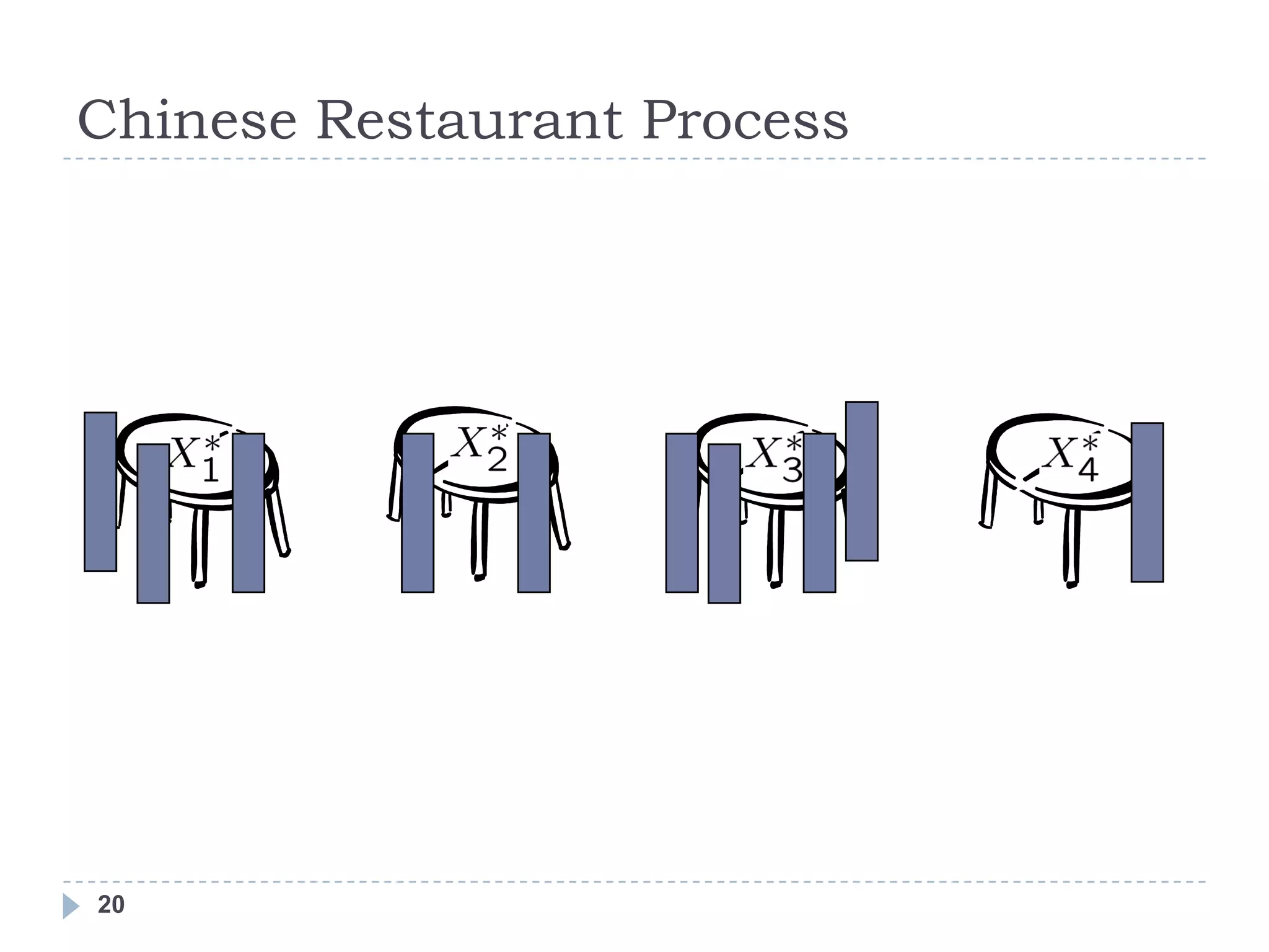
![Chinese Restaurant Process
Consider a restaurant with infinitely many tables, where the Xn‘s
represent the patrons of the restaurant. From the above
conditional probability distribution, we can see that a customer is
more likely to sit at a table if there are already many people
sitting there. However, with probability proportional to α, the
customer will sit at a new table.
Also known as the ―clustering effect,‖ and can be seen in the
setting of social clubs. [Aldous]
19](https://image.slidesharecdn.com/dptutorial-1304430760-phpapp01/75/Gentle-Introduction-to-Dirichlet-Processes-19-2048.jpg)

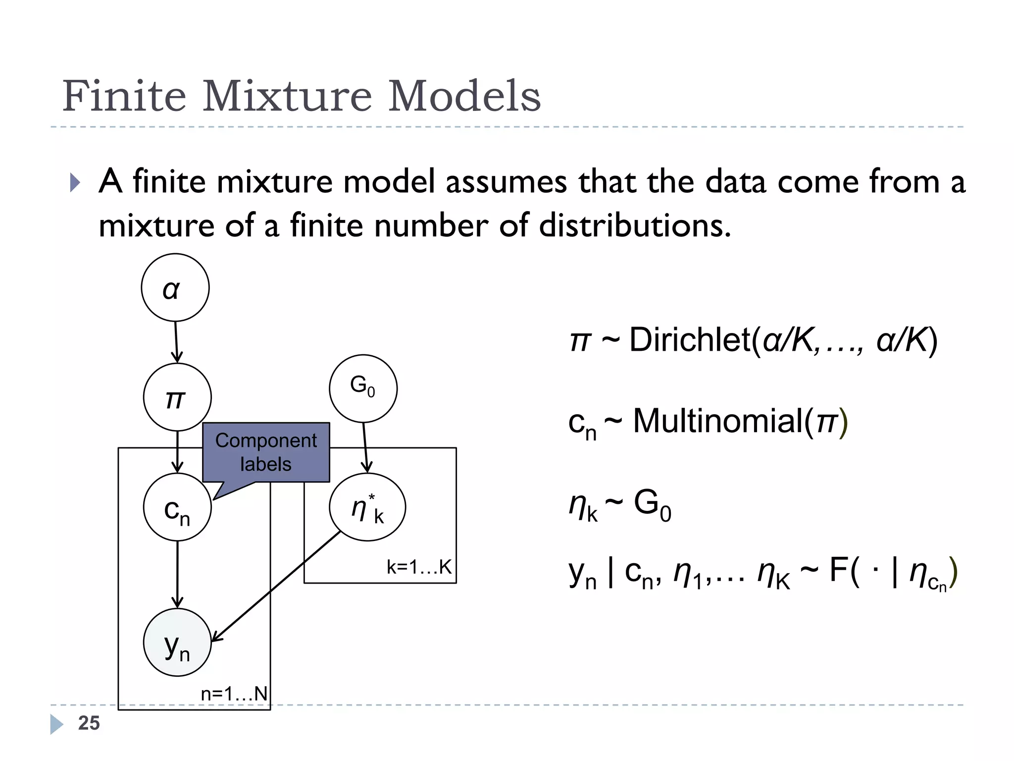
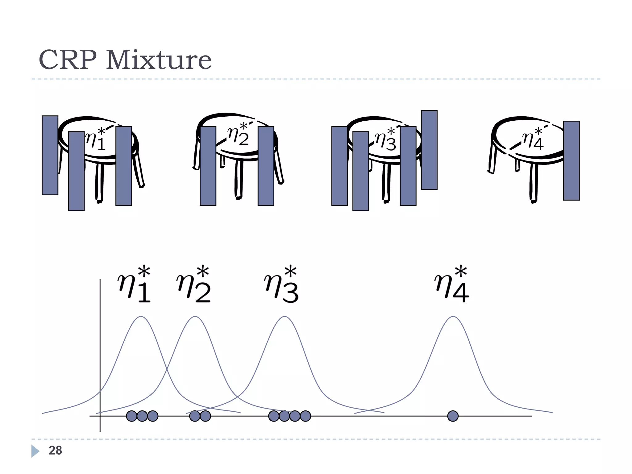
![Infinite Mixture Models
An infinite mixture model assumes that the data come
from a mixture of an infinite number of distributions
α
π ~ Dirichlet(α/K,…, α/K)
G0
π
cn ~ Multinomial(π)
cn η*k ηk ~ G0
k=1…K yn | cn, η1,… ηK ~ F( · | ηcn)
Take limit as K goes to ∞
yn
Note: the N data points still come from at most N
n=1…N
different components [Rasmussen 2000]
26](https://image.slidesharecdn.com/dptutorial-1304430760-phpapp01/75/Gentle-Introduction-to-Dirichlet-Processes-26-2048.jpg)
![Inference for Dirichlet Process Mixtures
Expectation Maximization (EM) G0
is generally used for inference in
G
a mixture model, but G is α
nonparametric, making EM
difficult
ηn
Markov Chain Monte Carlo
techniques [Neal 2000]
yn
Variational Inference [Blei and
Jordan 2006] n=1…N
30](https://image.slidesharecdn.com/dptutorial-1304430760-phpapp01/75/Gentle-Introduction-to-Dirichlet-Processes-30-2048.jpg)
![Aside: Monte Carlo Methods
[Basic Integration]
We want to compute the integral,
where f(x) is a probability density function.
In other words, we want Ef [h(x)].
We can approximate this as:
where X1, X2, …, XN are sampled from f.
By the law of large numbers,
[Lafferty and Wasserman]
31](https://image.slidesharecdn.com/dptutorial-1304430760-phpapp01/75/Gentle-Introduction-to-Dirichlet-Processes-31-2048.jpg)
![Aside: Monte Carlo Methods
[What if we don’t know how to sample from f?]
Importance Sampling
Markov Chain Monte Carlo (MCMC)
Goal is to generate a Markov chain X1, X2, …, whose stationary
distribution is f.
If so, then
N
1 X p
h(Xi) ¡! I
N i=1
(under certain conditions)
32](https://image.slidesharecdn.com/dptutorial-1304430760-phpapp01/75/Gentle-Introduction-to-Dirichlet-Processes-32-2048.jpg)
![Aside: Monte Carlo Methods
[MCMC I: Metropolis-Hastings Algorithm]
Goal: Generate a Markov chain with stationary distribution f(x)
Initialization:
Let q(y | x) be an arbitrary distribution that we know how to sample
from. We call q the proposal distribution.
A common choice
Arbitrarily choose X0. N(x, b2) for b > 0
is
If q is symmetric,
Assume we have generated X0, X1, …, Xi. To generate
simplifies to:
Xi+1:
Generate a proposal value Y ~ q(y|Xi)
Evaluate r ≡ r(Xi, Y) where:
Set:
with probability r
with probability 1-r
33 [Lafferty and Wasserman]](https://image.slidesharecdn.com/dptutorial-1304430760-phpapp01/75/Gentle-Introduction-to-Dirichlet-Processes-33-2048.jpg)
![Aside: Monte Carlo Methods
[MCMC II: Gibbs Sampling]
Goal: Generate a Markov chain with stationary distribution
f(x, y) [Easily extendable to higher dimensions.]
Assumption:
We know how to sample from the conditional distributions
fX|Y(x | y) and fY|X(y | x) If not, then we run one iteration
Initialization: of Metropolis-Hastings each
time we need to sample from a
Arbitrarily choose X0,Y0. conditional.
Assume we have generated (X0,Y0), …, (Xi,Yi). To
generate (Xi+1,Yi+1):
Xi+1 ~ fX|Y(x | Yi)
Yi+1 ~ fY|X(y | Xi+1)
34 [Lafferty and Wasserman]](https://image.slidesharecdn.com/dptutorial-1304430760-phpapp01/75/Gentle-Introduction-to-Dirichlet-Processes-34-2048.jpg)
![MCMC for Dirichlet Process Mixtures
[Overview]
We would like to sample from the
posterior distribution: G0
P(η1,…, ηN | y1,…yN) G
If we could, we would be able to α
determine:
how many distinct components are likely
contributing to our data. ηn
what the parameters are for each
component.
[Neal 2000] is an excellent resource yn
describing several MCMC algorithms
for solving this problem. n=1…N
We will briefly take a look at two of them.
35](https://image.slidesharecdn.com/dptutorial-1304430760-phpapp01/75/Gentle-Introduction-to-Dirichlet-Processes-35-2048.jpg)
![MCMC for Dirichlet Process Mixtures
[Infinite Mixture Model representation]
MCMC algorithms that are based
on the infinite mixture model α
representation of Dirichlet Process
Mixtures are found to be simpler to G0
implement and converge faster than π
those based on the direct
representation.
cn η*k
Thus, rather than sampling for η1,…,
ηN directly, we will instead sample k=1…∞
for the component indicators c1, …,
cN, as well as the component yn
parameters η*c, for all c in {c1, …, n=1…N
cN}
[Neal 2000]
36](https://image.slidesharecdn.com/dptutorial-1304430760-phpapp01/75/Gentle-Introduction-to-Dirichlet-Processes-36-2048.jpg)
![MCMC for Dirichlet Process Mixtures
[Gibbs Sampling with Conjugate Priors]
Assume current state of Markov chain consists of c1, …, cN,
as well as the component parameters η*c, for all c in {c1, …,
cN}.
To generate the next sample:
1. For i = 1,…,N:
If ci is currently a singleton, remove η*ci from the state.
Draw a new value for ci from the conditional distribution:
for existing c
for new c
If the new ci is not associated with any other observation,
draw a value for η*ci from: [Neal 2000, Algorithm 2]
37](https://image.slidesharecdn.com/dptutorial-1304430760-phpapp01/75/Gentle-Introduction-to-Dirichlet-Processes-37-2048.jpg)
![MCMC for Dirichlet Process Mixtures
[Gibbs Sampling with Conjugate Priors]
2. For all c in {c1, …, cN}:
Draw a new value for η*c from the posterior distribution
based on the prior G0 and all the data points currently
associated with component c:
This algorithm breaks down when G0 is not a conjugate
prior.
[Neal 2000, Algorithm 2]
38](https://image.slidesharecdn.com/dptutorial-1304430760-phpapp01/75/Gentle-Introduction-to-Dirichlet-Processes-38-2048.jpg)
![MCMC for Dirichlet Process Mixtures
[Gibbs Sampling with Auxiliary Parameters]
Recall from the Gibbs sampling overview: if we do not know
how to sample from the conditional distributions, we can
interleave one or more Metropolis-Hastings steps.
We can apply this technique when G0 is not a conjugate prior, but it
can lead to convergence issues [Neal 2000, Algorithms 5-7]
Instead, we will use auxiliary parameters.
Previously, the state of our Markov chain consisted of c1,…, cN,
as well as component parameters η*c, for all c in {c1, …, cN}.
When updating ci, we either:
choose an existing component c from c-i (i.e., all cj such that j ≠ i).
choose a brand new component.
In the previous algorithm, this involved integrating with respect to G0,
which is difficult in the non-conjugate case.
[Neal 2000, Algorithm 8]
39](https://image.slidesharecdn.com/dptutorial-1304430760-phpapp01/75/Gentle-Introduction-to-Dirichlet-Processes-39-2048.jpg)
![MCMC for Dirichlet Process Mixtures
[Gibbs Sampling with Auxiliary Parameters]
When updating ci, we either:
choose an existing component c from c-i (i.e., all cj such that j ≠ i).
choose a brand new component.
Let K-i be the number of distinct components c in c-i.
WLOG, let these components c-i have values in {1, …, K-i}.
Instead of integrating over G0, we will add m auxiliary
parameters, each corresponding to a new component
independently drawn from G0 :
[η*K +1 , …, η*K-i +m ]
-i
Recall that the probability of selecting a new component is proportional to α.
Here, we divide α equally among the m auxiliary components.
[Neal 2000, Algorithm 8]
40](https://image.slidesharecdn.com/dptutorial-1304430760-phpapp01/75/Gentle-Introduction-to-Dirichlet-Processes-40-2048.jpg)
![MCMC for Dirichlet Process Mixtures
[Gibbs Sampling with Auxiliary Parameters]
Probability: 2 1 2 1 α/3 α/3 α/3
(proportional to)
Components: η*1 η*2 η* 3 η*4 η*5 η* 6 η*7
Each is a fresh draw from G0
Data: y1 y2 y3 y4 y5 y6 y7
cj: 1 2 1 3 4 3 ?
This takes care of sampling for ci in the non-conjugate case.
A Metropolis-Hastings step can be used to sample η*c.
See Neal‘s paper for more details.
[Neal 2000, Algorithm 8]
41](https://image.slidesharecdn.com/dptutorial-1304430760-phpapp01/75/Gentle-Introduction-to-Dirichlet-Processes-41-2048.jpg)

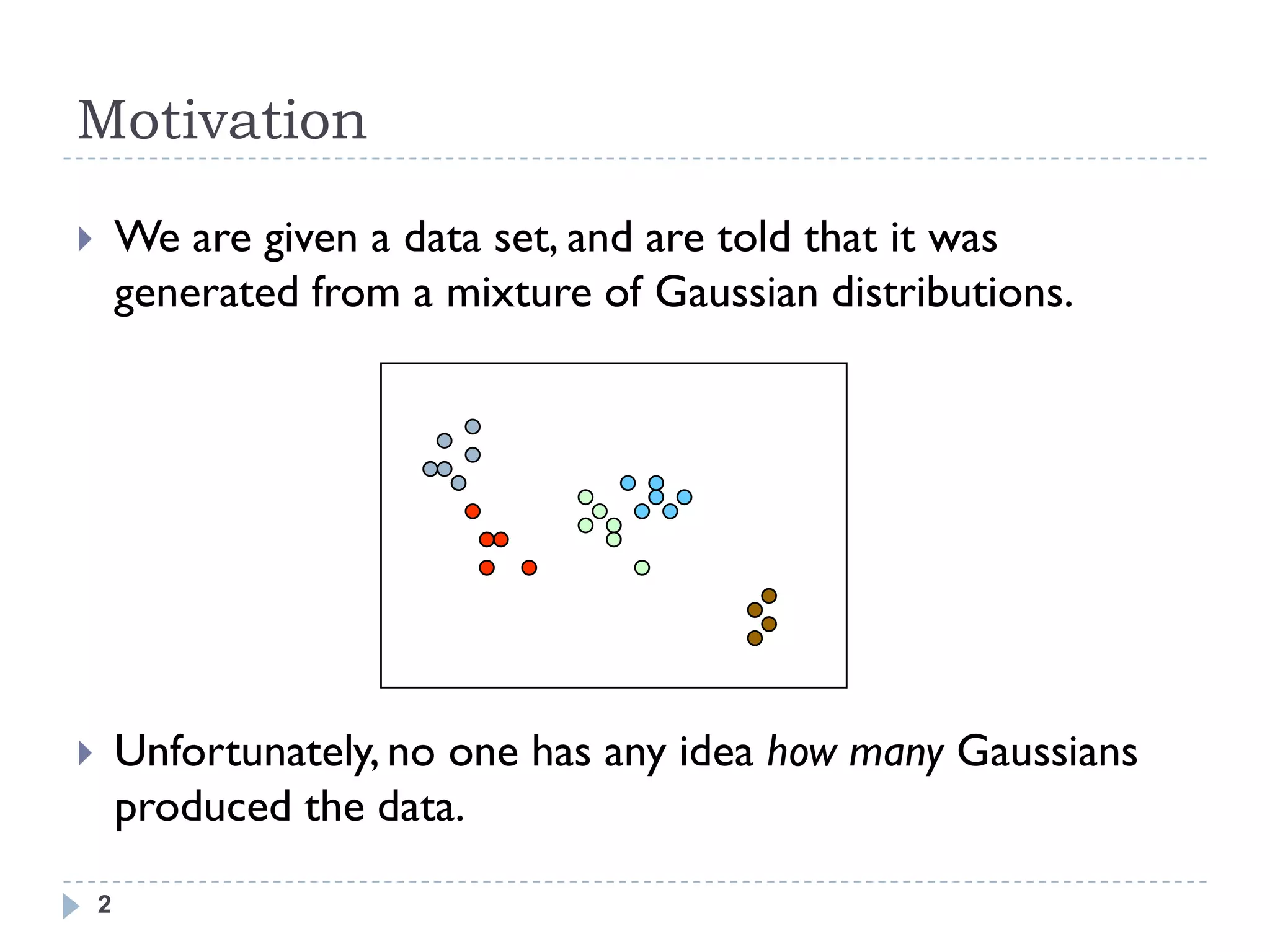
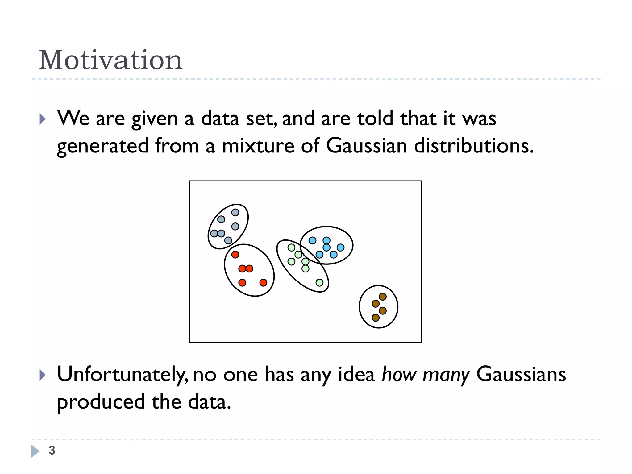
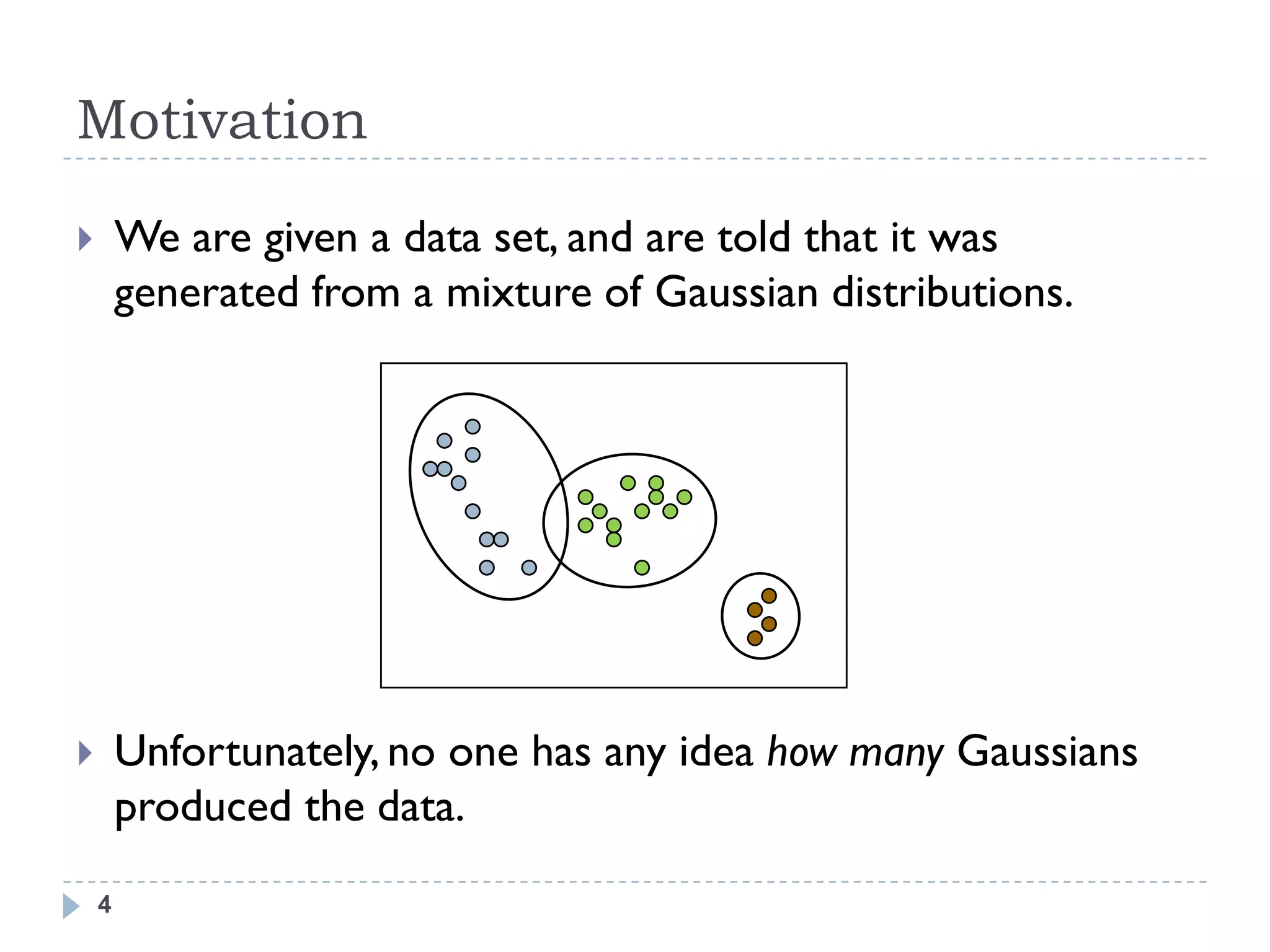
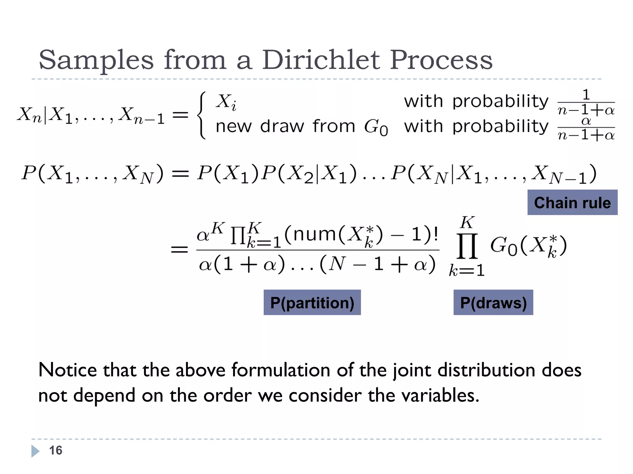
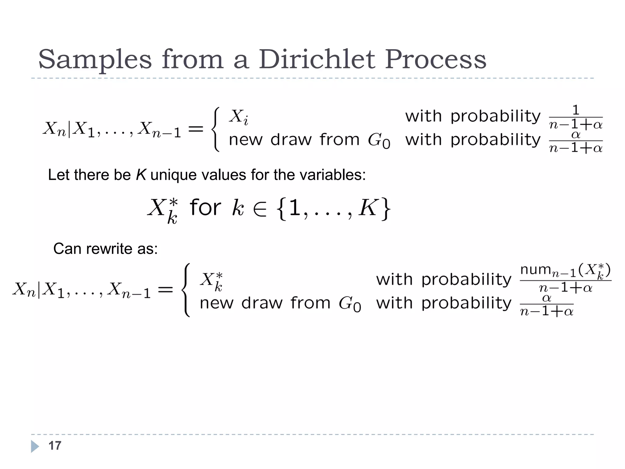
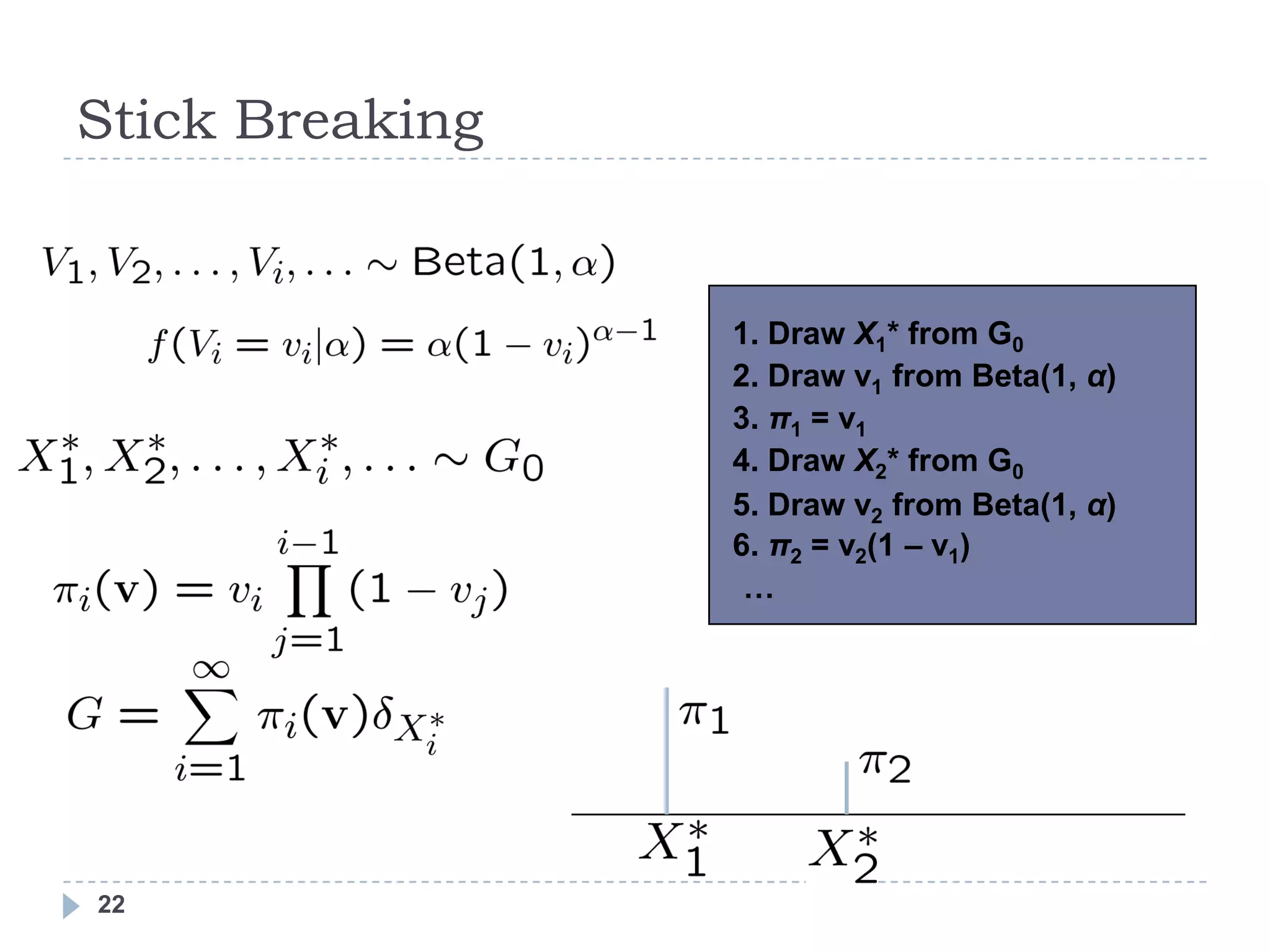
This document provides an introduction to Dirichlet processes. It begins by motivating the need for nonparametric clustering when the number of clusters in the data is unknown. It then provides an overview of Dirichlet processes and discusses them from multiple perspectives, including samples from a Dirichlet process, the Chinese restaurant process representation, stick breaking construction, and formal definition. It also covers Dirichlet process mixtures and common inference techniques like Markov chain Monte Carlo and variational inference.