Download as PDF, PPTX

![Bayesian Portfolio Analysis
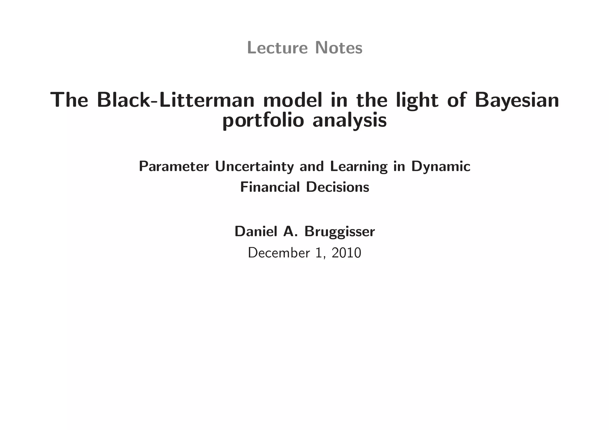
• The classical portfolio selection problem:1
max ET [U (WT +1)] = max U (WT +1)p(rT +1|θ)drT +1 (1)
ω ω Ω
f f
s.t. WT +1 = WT ω ′ exp(rT +1 + rT ) + (1 − ι′ω) exp(rT ) , (2)
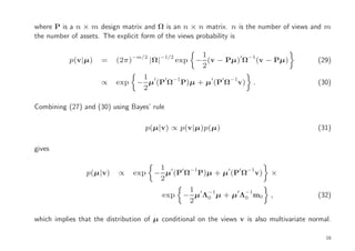
where Ω is the sample space, U (WT +1) is a utility function, WT +1 is the wealth
at time T + 1, θ is a set parameters, ω are portfolio weights, p(rT +1|θ) is the
f
sample density of returns, rT is the risk free rate, and ι is a vector of ones. The
column vectors ι, ω and rT +1 are of the same dimension.
• The parameter vector θ is assumed to be known to the investor. However, some
parameters are estimates and subject to parameter uncertainty.
4](https://image.slidesharecdn.com/ppbl01-111005072917-phpapp01/85/The-Black-Litterman-model-in-the-light-of-Bayesian-portfolio-analysis-4-320.jpg)
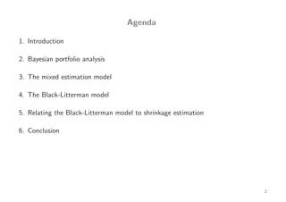
![• Bayesian portfolio selection problem:2
max ET [U (WT +1)] = max U (WT +1)p(rT +1|ΦT )drT +1, (3)
ω ω Ω
f f
s.t. WT +1 = WT ω ′ exp(rT +1 + rT ) + (1 − ι′ω) exp(rT ) , (4)
where ΦT is the information available up to time T , and p(rT +1|ΦT ) is the
Bayesian predictive distribution (density) of asset returns.
• Conditioning takes place on ΦT instead of essentially uncertain parameters θ.
• There are many ways to derive the Bayesian predictive distribution depending on
the model at hand, the choice of the prior distribution of uncertain quantities, and
the information the investor assumes as known.
5](https://image.slidesharecdn.com/ppbl01-111005072917-phpapp01/85/The-Black-Litterman-model-in-the-light-of-Bayesian-portfolio-analysis-5-320.jpg)
![• Bayesian decomposition, Bayes′ rule and Fubini′s theorem:3
ET [U (WT +1)] = U (WT +1)p(rT +1|ΦT )drT +1 (5)
Ω
= U (WT +1)p(rT +1, θ|ΦT )d(drT +1, θ)
Ω×Θ
= U (WT +1)p(rT +1|θ)p(θ|ΦT )dθdrT +1
Ω Θ
= U (WT +1) p(rT +1|θ)p(ΦT |θ)p(θ)dθ drT +1,
Ω Θ
where Θ is the parameter space, p(rT +1, θ|ΦT ) is the joint density of parameters
and realizations, p(θ|ΦT ) is the posterior density, p(ΦT |θ) is the conditional
likelihood, and p(θ) is the prior density of the parameters.
6](https://image.slidesharecdn.com/ppbl01-111005072917-phpapp01/85/The-Black-Litterman-model-in-the-light-of-Bayesian-portfolio-analysis-6-320.jpg)
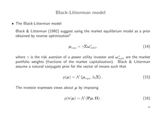
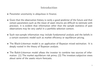
![Relating the Black-Litterman model to shrinkage estimation
• The Black-Litterman model can be aligned to shrinkage estimation by matrix
algebra.7
If P and Ω are m × m with full rank (n = m), and v is an m × 1 vector, the
mean of the posterior in (18) can be written in shrinkage form:
µv = δµequ + (I − δ)(P′P)−1 P′v, (22)
where I is an m × m identity matrix with principal diagonal elements of one and
zero elsewhere. δ is called the posterior shrinkage factor. It can be shown that8
−1
−1
δ = (λ0Σ) ′
+PΩ −1
P (λ0Σ)−1 (23)
−1
= [prior covariance]−1 + [conditional covariance]−1 [prior covariance]−1
= [posterior covariance][prior covariance]−1.
12](https://image.slidesharecdn.com/ppbl01-111005072917-phpapp01/85/The-Black-Litterman-model-in-the-light-of-Bayesian-portfolio-analysis-12-320.jpg)
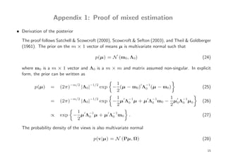
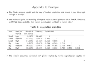
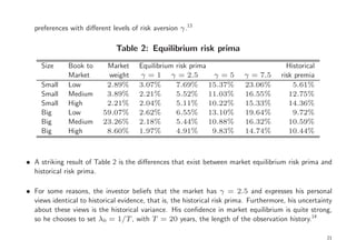
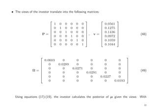
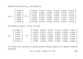
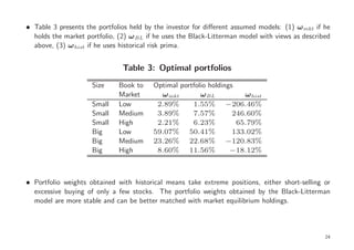

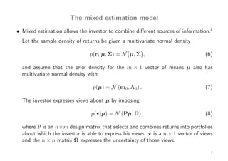
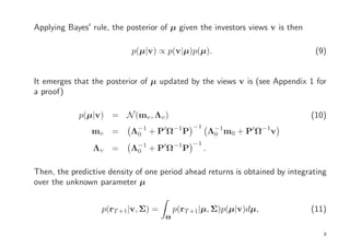
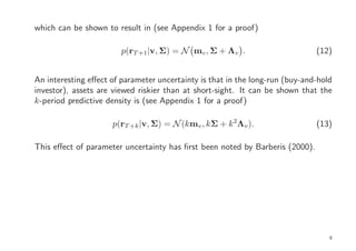
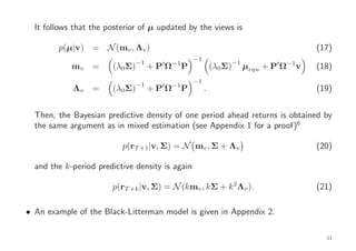
The document discusses the Black-Litterman model in the context of Bayesian portfolio analysis, exploring how parameter uncertainty affects financial decision-making. It emphasizes the integration of market equilibrium risk premia with investors' subjective views on asset returns, highlighting the advantages of using the mixed estimation model. The Black-Litterman model enhances portfolio stability by enabling investors to incorporate non-sample information, contrasting with traditional portfolio selection based solely on past observations.