Tensor Decomposition and its Applications

Applications of tensor
(multiway array)
factorizations and
decompositions in data mining

機械学習班輪講
11/10/25
@taki__taki__

Paper

Mørup, M. (2011), Applications of
tensor (multiway array) factorizations
and decompositions in data mining.
Wiley Interdisciplinary Reviews: Data
Mining and Knowledge Discovery, 1: 24–
40. doi: 10.1002/widm.1

こちらの論文からいくつか図を引用します．

Table of Contents

1.全体のイントロダクション
2.2階のテンソルと行列分解
3.SVD: Singular Value Decomposition
4.論文のイントロダクションと記法など
5.TuckerモデルとCPモデルの紹介
6.応用とまとめ

Introduction
• テンソル分解(本文中ではfactorization，又は
decomposition)がデータマイニングの分野で重要
な道具になってきているため，紹介する
• (Wikipediaでは)テンソル(tensor)とは線形的
な量または幾何概念を一般化したもの
→乱暴に言えば多次元配列に相当する
• 主に行列(2階のテンソル)と，3次元配列(3階の
テンソル，複数の行列の集まり)を題材として
テンソル分解を考える

まずは行列分解から考える

2階のテンソル (1)
• 定義: 2つの任意のベクトルに対して実数
を対応させる関数で，任意のベクトル及
びスカラーkに対して以下の双線形性が成り立つ
関数Tを2階のテンソルと呼ぶ

• ベクトルの内積は関数Tになる．正規直交
基底上の3次元空間において，基底ベ
クトルに対するテンソルをとする

• {i,j}の組合せに対応して
任意のベクトルu, v

基本ベクトルの変換対
• 双線形性より

• 行列による線形変換は基本ベクトルの変換対と
同じ形になるので，2つを対応させて考える

• 任意のベクトル
たベクトル
を線形変換Tで変換させ
の成分はTの行列表示
を用いて表現できる (普通の行列の積)
• 行列の線形変換は2つのベクトルv,uに対して次
の線形性を持つ:
• ベクトルvの線形変換Tによる像T(v)と，ベクト
ルuとの内積が実数なので，この操作を関数と
して置く:
• これは双線形性を満たすので，このTを新しく2
階のテンソルとする．そこで2階のテンソルを
行列Tでも表現することとする．

2階のテンソルの分解 (1)
• 例えばグラフは隣接行列という形で表現された
り，文章と単語の出現関係を行列で表現した
り，行列表現は比較的良く出てくる
• そこで行列の特性を測ったり，特徴を表現した
りする技術に線形代数での技術を用いる

変換
分解

データの世界線形代数の世界

2階のテンソルの分解 (2)
• 2階のテンソルが行列で表現されるため，2階の
テンソル分解は行列分解同値．そこで特異値分
解(SVD:Singular Value Decomposition)を例題
として見る．
• SVDは行列分解として基本的な操作の一つで，
LSI(Latent Semantic Indexing)で利用されて
いる．LSIでは各文書における単語の出現を表
して行列を利用する．
• 単語iが文書jに出現するとき，行列の(i,j)要素にその情報
を入れる:(頻度，出現回数，TF-IDFの情報，etc)

• SVDはこの行列を用語と何らかの概念の関係及
び概念と文書間の関係に変換する

SVD:Singular Value Decomposition
• SVDの考え方は次のようになる．例として文書
と単語の出現に関する行列Xを考える．
各文書djにおける
各単語tiの情報

各単語tiの
各文書djの情報

は単語ベクトル同士の内積全てが入る
は文書ベクトル同士の内積全てが入る

• SVDの考え方は次のようになる．例として文書
と単語の出現に関する行列Xを考える．
は単語ベクトル同士の内積全てが入る
は文書ベクトル同士の内積全てが入る

• 仮に行列Xが直交行列U，Vと対角行列Σによっ
て分解されるならば…

が対角行列
単語に関する情報はUに，文章に関する情報はVに入る

• SVDは(m,n)行列Aをに分解する
• U: (m,r)行列．行列のr個の非零な固有
ベクトル(左特異)から構成される．
• V: (n,r)行列．行列のr個の非零な固有
ベクトル(右特異)から構成される．
• Σ:(r,r)行列．特異値からなる対角行列．特
異値はの非零な固有値の降順にr個．
• SVDは重要ではない次元を自動的に落としてく
れる．そしてΣは元になった行列Aを上手く近
似してくれるとされる．

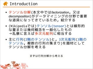
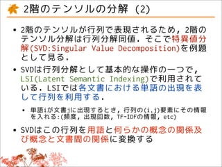
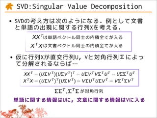
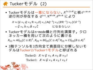
octave-3.4.0:4> A = [1 2 3; 4 5 6; 7 8 9];
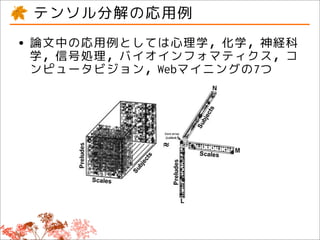
octave-3.4.0:5> [u v d] = svd(A);
octave-3.4.0:6> u
-0.21484 0.88723 0.40825
-0.52059 0.24964 -0.81650
-0.82634 -0.38794 0.40825

octave-3.4.0:7> v
1.6848e+01 0 0
0 1.0684e+00 0
0 0 1.4728e-16

octave-3.4.0:8> d
-0.479671 -0.776691 0.408248
-0.572368 -0.075686 -0.816497
-0.665064 0.625318 0.408248

論文のIntroduction
• (Wikipedia)テンソル(tensor)は，乱暴に言え
ば多次元配列に相当．2階のテンソル(行列)は2
次元配列，3階のテンソルは3次元配列である．
• 2階テンソルの例のように，色んなデータが3次
元以上の配列で集められているとする．そこで
SVDのように，そのテンソルをいくつかの要素
に分解して解釈したい．
• 論文ではCandecomp/Parafac(CP)モデルと，
Tuckerモデルと呼ばれるテンソル分解について
説明する．(自由度が高く，他にたくさんある)

eimportant framework for of modern large-by more,...,i N . The following sectiona in-operations that, for
. Tensor decompositiontypes applied denoted to xtroduces the basic notation and
discovery of many is being X is tation i 1 ,i 2 compactly denote the size of tensor
anthe opti- is sors, andtroduces is basicclarity, is 2given two tensors are
veryimportant framework thatthe X X product between for third-orderfor
g typesand modern large- for ten- inner
ny year of there no doubt
sets. I1denoted by xi ,i ,...,i . The following section in-
the ×I2 ×...×IN
notation and N element of the tensor whereas they
, whereas a given operations that, tensors,
テンソルに関する記法 (1)
decomposi- modern large- for troduces the third-orderNtensors, whereas they in- for
on will be an of has many challenges given for basici1 ,igeneralize following section that, order.
many typesimportant framework
or factorization given by clarity, is and
1
X is denoted by x notation andtensors of arbitrary
trivially 2 ,...,i . The to operations
has manythe types because its geometry isis given fornotation and operations that, for they ×K and
covery of many
particularly of modern large- clarity,
lems,on challenges and
ture
troduces the basic third-order third-order tensor
trivially generalize to tensors of arbitrary order. whereas A I×J
Consider the tensors,
.
on because its geometry is and of= C,
lly has many challenges
y understood, the occurrence αB degener-where forcthird-order tensors, whereasaddition of two ten-
Consider is given ×K toj,k = multiplication, (1)
clarity,
trivially generalize .i, Scalar αbi, j,k I×J ×K and
the I×J tensors of arbitrary order.
B third-order tensor A
they

s, • N階の実テンソルを
bit occurrence of degener- finding ×K . trivially generalize to third-order tensorbetween two tensors are
a because its geometry B
strong
actorization has many challenges and

the of finding
素を
と表し，各要
arly and no because its geometry is
ons,
と表す．簡単な例として3階のテン
Consider and
tensors of arbitrary order.
Scalar sors,the third-order tensor A I×J ×KI×J ×K
he particularly guarantee of is I×J the opti- multiplication, addition of two ten-and and
Consider the the inner product A
mitations a occurrence of degener- andBthe×K .Scalar multiplication, addition of two ten- ten-
antee occurrence most tensor decomposi-inner product between two tensors are two
on. Furthermore, of opti-
,nderstood, the the degener- sors, B I×JI×J . Scalar multiplication, addition of
×K given by
uarantee of very of findingopti-opti- sors, the where product= ai + bi tensors are αb are
rlsdecompo- decomposi- the given =on and the inner ci, j,k between two two (2)
most guarantee restricted A + B by sors, and the inner product between
impose a finding the structure C,
,and no tensor
αB = C, where ci, j,k = i, j,k
tensors (1)
ソル
h in turn structuredecomposi-
restricted tensor tensor decomposi- a strongby
Furthermore, most on the を考え，αを実数とする．
ore, mostrequire that data exhibit given by C, where ci, j,k = αbi, j,k
r the years. given
αB = (1)
mposedata exhibit a strong
that a very restricted structure on the
regularity. Tostructure on the limitations a αB = C, where ci, j,k = αbi, j,k
overcome these
ry restricted
process is スカラー倍
ercome these limitations of tensor decompo- αB = C, i, j,kbi, j,k C, ci, j,k = αbi, c(3) = ai + bi
a A+B =
A, B = (1)
re that data •
turn requireand variants a a strong
that data exhibit
extensions exhibit a strong
rlarity. Tohave been these limitations athe years.= C, i, j,k
decompo-
roaches overcome proposed over
riants of tensor decompo- A+B
where
where ci, j,k = ai + bi
where j,k j,k i,
(2)
(1) (2)

erstanding •
nsions and over テンソルの和
n proposed thesethe tensor
overcomevariants limitations a
herent mul-proposed over decompo-
of years. A + B = C, where ci, j,k = ai + bi
hes have beenthe data generating process is + B = C, of where Bci, j,kgiven byj,k
As such, √ Frobenius norm ai,a tensor = = ai, j,kbi,i
the A A,
is ai + b
(2)
(2) (3)
•
variants of tensor decompo-
formulation ofテンソルの内積
adequate
een proposed decompo- =
the years.
eata generating generating process is
process is tensor
anding the data over the years. decompo-
tensor extract the inherent .
adequate of adequate tensor decompo- A mul-
A F A,
A, B =
A, B =
i, j,k
j,kbi, j,k
ai, j,kbi, j,k i, j,k
(3)
(3)
dels that ten-well
mulation can
basic the inherentprocess is th
data well extract mul-The n As such, √= j,k ai, j,kb j,k
i,
e extractgenerating the inherent mul- mode matricizing and Frobeniusi,norm of a tensor is given by
A, B the unmatricizing op- (3)
ructure.
that can As such,As such, theA norm normtensor is given by by
the Frobenius = of a of a tensor is given
ure.
overview will •
andecomp/ limitdecompo- basic√ten-
of adequate tensorフロベニウスノルム√ Frobenius A,and a matrix into
itself to the F a tensor into AF matrixi, j,k
eration maps = A A,= . A, a .The nth mode matricizing and
A A
A.
rview will ap- basic the basic ten- The nthFmode matricizing and unmatricizing op- unmatricizing op-
• テンソルの行列化/非行列化
as their to theitself to ten- mul-Candecomp/The nth mode matricizing and unmatricizing op-
mit extract
ell itself models such as the
position
troductory
CP) and
limit inherent
such asTucker asathe as well as As such, the Frobenius norm of a tensor is given by
tensor, respectively, i.e.,
ition models suchmodel, Candecomp/ their ap- √ eration maps a tensor into a matrix and a matrix into
the Candecomp/
and Tucker model, their ap- ten- ap- A F =
eration maps a into into a matrix(n)番目を中心に開く
eration maps a tensorA . a matrix and a matrix intointo
A, tensor
model, asmining.the well as theirintroductory respectively,respectively, i.e.,
as basic
well as Other great a tensor, and a matrix
eirdataitselfOther great introductory N arespectively, i.e.,n ×Ii.e., ···In−1 ·In+1 ···Iunmatricizing op-
n mining. to
limit
ata applica-introductory ×I2 ×...×I
I1 a tensor, tensor, nth mode matricizing and N
→
The I 1 ·I2
Other great the Candecomp/
els tensoras
or such the decomposition X and their applica- X ×I2 ×...×IN → (4)
Ref 24
position and their applica- matricizingX I1 (n) n ×I1 X2I···Imatrix and(n) matrix into
→ → ·I n n−1 2 n+1 ···IN X a
···I
In
ensor decomposition and their applica- eration1 ×I2 ×...×Ia tensorIinto a×I1 ·I·I n−1 ·In+1 ···IN×I1 ·I2 ···In−1 ·In+1 ···IN
I maps N (4)
bemodel, in28well as their ap- theI1 ×I24 X N
r found asthe recent of Ref 24 X 2 ×...×I
ound in the recent review review of Ref the X (n) matricizing
matricizing (n) (4) (4)
lultiway analysis introductory 28 a tensor,matricizing i.e.,
sciences for thefor the chemical sciences28 respectively,
ecent review of Ref 24 the
g. Other greatsciences×Isciences ·In+1 ···IN
way analysis chemical 1 ·I2 ···In−1
In 28 → ···I n+1
for the chemical
the book
book on applied X applica- analysis(n)×I ·I2 ···INX In ···I ·I2→ → I1 IN1×IX·II21···I2→ ·In+1 ···IN
analysis on applied (n) analysis Iof 1 ·I2 ···IIn−1 ·I1n+1···In−1 ·I(n)×I1N → n−1 ·IX ···I×I2 ×...×I×...×IN(5) X I1 ×I2 ×...×IN (5)
of multiway In
mposition and their multiway n ×I X 1 ofun-matricizing X I ×I12 ×...×IN (5) (5)
n+1 ×I N
plied multiway analysis of nonnega- X ×I2 ×...×IN
X (n) un-matricizing
X (n) un-matricizing
n n−1
(4)
orecent review ofintroduction
nonnega-
more, a good introduction to
e introduction to nonnega- the to nonnega-
thermore, a good Ref 24 un-matricizing
matricizing
d and decompositions can be foundbe found in
s their the chemical sciences28 in The matricizing matricizing operation for a
The operation for a third-order tensor is
be for theircan model estimation The matricizing operation a third-order tensorisisof
is found in be found in can re- illustrated in Figure for a third-order tensor third-order tensor is
mpositions
decompositions
present paper, The matricizing operation for 1. The n-mode multiplication
is
the present paper,analysis of →
model estimation Iis re- 2 ···In−1 ·In+1 ···IN I1 ×I2 ×...×IN 1. The I1 ×I2 ×...×IN (5)
multiway illustrated and Figure·I1. Nillustrated in Figure a matrix M J ×Inmultiplication of
appliedis estimation is re-
ation
r, model re-
nimum considering only the simple in
n ×I1
X anin Figuretensor X n-mode multiplication of
illustrated order The n-mode multiplication of
1. The with X n-mode

The n mode matricizing and unmatricizing op-
s the Candecomp/
eration maps a tensor into a matrix and a matrix into
行列化のイメージ
as well as their ap-
great introductory
a tensor, respectively, i.e.,
n and their applica- → In ×I ·I ···I ·I ···I
Overview X I1 ×I2 ×...×IN X (n) 1 2 n−1 n+1 N (4) wires.wiley.com/widm
view of Ref 24 the matricizing
chemical sciences28
In ×I ·I ···I ·I ···I →
ultiway analysis of X (n) 1 2 n−1 n+1 N X I1 ×I2 ×...×IN (5)
un-matricizing
uction to nonnega-
(3)
ons can be found in The matricizing operation for a third-order tensor is
el estimation is re- illustrated in Figure 1. The n-mode multiplication of
only the simple and (2) an order N tensor X I1 ×I2 ×...×IN with a matrix M J ×In
res (ALS) approach. is given by
sor model estima-
the reader consult X ×n M = X •n M = Z I1 ×...×In−1 ×J ×In+1 ×...×IN , (6)
s therein. In
ollows: In ‘Tensor
zi1 ,...,in−1 , j,in+1 ,...,i N = xi1 ,...,in−1 ,in ,in+1 ,...,i N m j,in . (7)
andard tensor no-
i n =1
ucker and Cande-
ibe(1) two most
the Using the matricizing operation, this operation cor-
approaches namely responds to Z(n) = MX (n) . As a result, the matrix
ns as well as some products underlying the singular value decomposi-
torization for Data tion (SVD) can be written as U SV = S ×1 U ×2 V =
applications 1 | The matricizing S ×2 V ×third-order tensor oforder 4of 4. multiplication does
F I G U R E of ten- operation on a
1 U as the size 4 × × the
on in data mining. not matter. The outer product of the three vectors a,
whereas the Khatri–Rao product is deﬁned as a to O(max{I J 2 , K J 2 , J 3 , L3 })(本文中より引用)
and O(I K J 2 ) to
m ofcolumn-wise Kroneckerb, and c is given by
this article is product 2 2 3
O(max{I K J, I J , K J , J }), respectively. For addi-

• n-mode積: テンソル
mode積は
と行列のn-
と表記する．定義は次
のようになる．

行列化演算子を用いて
行列AのSVD: はn-mode積を用いて

n-mode積の定理/性質らしい

• ベクトル3つの外積は3階のテンソルを成す
• クロネッカー積
• Khatri-Rao積 (column-wise クロネッカー積)

ムーアペンローズの逆行列を求めるとき

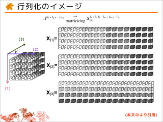
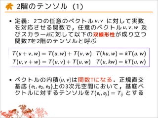
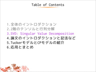
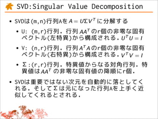
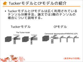
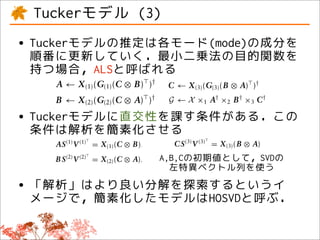
Penrose inverse (i.e., A = ( A A) A ) of Kronecker
and Khatri–Rao products are THE TUCKER AND
CANDECOMP/PARAFAC MODELS
( P ⊗ Q)† = ( P † ⊗ Q† ) (11)
The two most widely used tensor decomposition
methods are the Tucker model29 and Canonical De-
(A B)† = [( A A)∗ (B B)]−1 ( A B) (12)
composition (CANDECOMP)30 also known as Parallel
where ∗ denotes elementwise multiplication. Factor Analysis (PARAFAC)31 jointly abbreviated CP.
This reduces the complexity from O(J 3 L3 ) In the following section, we describe the models for

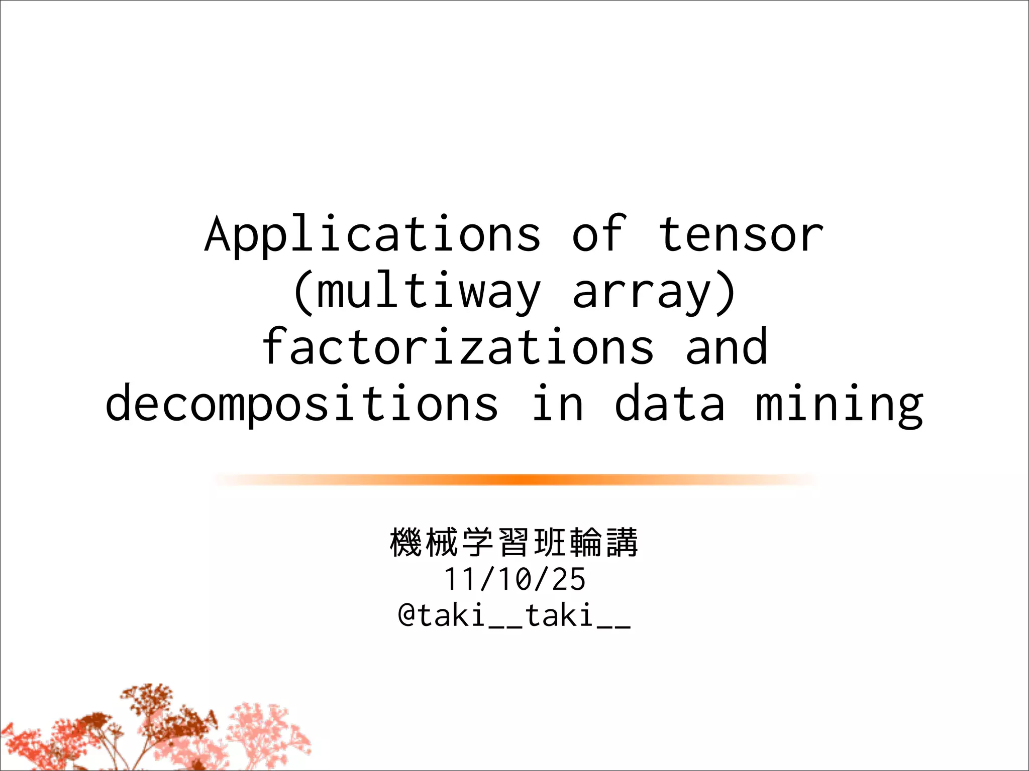
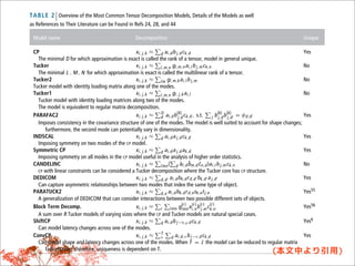
T A B L E 1 Summary of the Utilized Variables and Operations. X , X, x, and x are Used to Denote
Tensors, Matrices, Vectors, and Scalars Respectively.

Operator Name Operation

A, B Inner product A, B = i , j ,k a i , j ,k bi , j ,k
√
A F Frobenius norm A, A
I n × I · I ··· I · I ··· I
X(n ) Matricizing X I 1 × I 2 ×...× I N → X (n ) 1 2 n −1 n +1 N
×n or •n n-mode product X ×n M = Z where Z(n ) = MX (n )
◦ outer product a ◦ b = Z where z i , j = a i b j
⊗ Kronecker product A ⊗ B = Z where z k + K (i −1),l + L ( j −1) = a i j bkl
or | ⊗ | Khatri–Rao product A B = Z, where z k + K (i −1), j = a i j bk j .
kA k-rank Maximal number of columns of A guaranteed to be linearly independent.

26 c 2011 John Wiley & Sons, Inc. Volume 1, January/February 2011

(本文中より引用)

TuckerモデルとCPモデルの紹介
• TuckerモデルとCPモデルは広く利用されている
テンソル分解手法．論文では3階のテンソルの
場合について説明する．

Tuckerモデル
WIREs Data Mining and Knowledge Discovery
CPモデル
Applications of tensor (multiway array) factorizations and decompositions in data mining
WIREs Data Mining and Knowledge Discovery Applications o

multiplication by orthogonal/orthonormal matrices
Q, R, and S. Using the n-mode matricizing and an
Kronecker product operation, the Tucker model can ces
be written as cal
X (1) ≈ AG(1) (C ⊗ B) be
po
X (2) ≈ B G(2) (C ⊗ A)
tor
X ≈ CG (B ⊗ A) . rep
F I G U R E 2 | Illustration of the Tucker model of a third-order tensor F I G U R E 3 |(3) (3)
Illustration of the CANDECOMP/PARAFAC (CP) model of a
X . The model decomposes the tensor into loading matrices with a
The third-order tensor X . The model decomposes a tensor into a sum of
above decomposition for a third-order tensor is
mode specific number of components as well as a core array also rank one components and the model is very appealing due to its
denoted a Tucker3 model, the Tucker2 model ap
accounting for all multilinear interactions between the components of and uniquenessmodels are given by
Tucker1 properties. cu
each mode. The Tucker model is particularly useful for compressing Tucker2: X ≈ G × 1 A ×2 B ×3 I , are
tensors into a reduced representation given by the smaller core array G . sol
R D×D, and S D×D, we find×2 I ×3 I ,
Tucker1: X ≈ G ×1 A ma
a third-order tensor but they trivially generalize to
where X ≈ the ×1 Q ×2 R ×3 S) ×1 (本文中より引用)
I is (D identity matrix. Thus, (the Tucker1(B R−1 )
A Q−1 ) ×2 to
general Nth order arrays by introducing additional
model is equivalent −1 regular matrix decomposition
to nu
mode-specific loadings. × (CS ) = D × A × B × C.

T A B L E 2 Overview of the Most Common Tensor Decomposition Models, Details of the Models as well
as References to Their Literature can be Found in Refs 24, 28, and 44

Model name Decomposition Unique

CP x i , j ,k ≈ d a i ,d b j ,d c k ,d Yes
The minimal D for which approximation is exact is called the rank of a tensor, model in general unique.
Tucker x i , j ,k ≈ l ,m ,n gl ,m ,n a i ,l b j ,m c k ,n No
The minimal L , M , N for which approximation is exact is called the multilinear rank of a tensor.
Tucker2 x i , j ,k ≈ l m gl ,m ,k a i ,l b j ,m No
Tucker model with identity loading matrix along one of the modes.
Tucker1 x i , j ,k ≈ l ,m ,n gl , j ,k a i ,l No
Tucker model with identity loading matrices along two of the modes.
The model is equivalent to regular matrix decomposition.
PARAFAC2 x i , j ,k ≈ d a i ,d b (jk ) c k ,d , s.t.
D
,d
(k ) (k )
j b j ,d b j ,d = ψd ,d Yes
Imposes consistency in the covariance structure of one of the modes. The model is well suited to account for shape changes;
furthermore, the second mode can potentially vary in dimensionality.
INDSCAL x i , j ,k ≈ d a i ,d a j ,d c k ,d Yes
Imposing symmetry on two modes of the CP model.
Symmetric CP x i , j ,k ≈ d a i ,d a j ,d a k ,d Yes
Imposing symmetry on all modes in the CP model useful in the analysis of higher order statistics.
CANDELINC ˆ ˆ
x i , j ,k ≈ l mn ( d al ,d bm ,d c n ,d )a i ,l b j ,m c k ,n
ˆ No
CP with linear constraints can be considered a Tucker decomposition where the Tucker core has CP structure.
DEDICOM x i , j ,k ≈ d ,d a i ,d bk ,d r d ,d bk ,d a j ,d Yes
Can capture asymmetric relationships between two modes that index the same type of object.
PARATUCK2 x i , j ,k ≈ d ,e a i ,d bk ,d r d ,e sk ,e t j ,e Yes55
A generalization of DEDICOM that can consider interactions between two possible different sets of objects.
Block Term Decomp. x i , j ,k ≈ r l mn gl(r ) a i(,n b (jr,)m c kr,)n
mn
r) (
Yes56
A sum over R Tucker models of varying sizes where the CP and Tucker models are natural special cases.
ShiftCP x i , j ,k ≈ d a i ,d b j −τi ,d ,d c k ,d Yes6
Can model latency changes across one of the modes.
T
ConvCP x i , j ,k ≈ τ d a i ,d ,τ b j −τ,d c k ,d Yes
Can model shape and latency changes across one of the modes. When T = J the model can be reduced to regular matrix
factorization; therefore, uniqueness is dependent on T. (本文中より引用)

Tuckerモデル (1)
• Tuckerモデルは3階のテンソル
(core-array)
を核配列
と3つのmodeに分ける．

n-mode積による定義
WIREs Data Mining and Knowledge Discovery Applications of tensor (multiway array) factorizations and decomp

multiplication by orthogonal/orthon
Q, R, and S. Using the n-mode m
Kronecker product operation, the Tu
be written as
X (1) ≈ AG(1) (C ⊗ B)
X (2) ≈ B G(2) (C ⊗ A)
X (3) ≈ CG(3) (B ⊗ A)
F I G U R E 2 | Illustration of the Tucker model of a third-order tensor
X . The model decomposes the tensor into loading matrices with a
The above decomposition for a third
mode speciﬁc number of components as well as a core array also denoted a Tucker3 model, the
and Tucker1 models are given by

Tuckerモデル (2)
• Tuckerモデルは一意にならない．により
逆行列が存在する
と核

になるらしい

• Tuckerモデルはn-mode積と行列化演算子，クロ
ネッカー積を用いて次のように書ける

• 3階テンソルを3方向全て真面目に分解しないモ
デルはTucker2/Tucker1モデルと呼ばれる

on the basis the solution of each is denoted solved Xfitting (C ⊗ B) )
A ← (1) (G(1)
entsminimization, of updating the elements be ALS. Bymode the model using ALS, the
of each mode. To indicate how mode can of each
Tuckerモデル (3)
ainin turn modality, it is customary estimation reducesX (2) (G(2) (C ⊗ A) of regular matrix
to each that for the least squares objective B ← to a sequence )
by pseudoinverses, i.e., commonly †
ai,l b j,mc Tucker(L, M, N) model. factorization problems. As a result, for least squares
,nmodel a k,n ,
e is denoted ALS. By fitting the model using ← X the (B ⊗ A) )†C ALS,(3) (G(3)
A ← X (1) (G(1) (C ⊗ B) )†
tensor product reduces the model minimization, the matrix †of each mode can be solved
to a sequence of regular solution × B † × C† .
29,32
estimation ×n ,
• Tuckerモデルの推定は各モード(mode)の成分を
re factorization problems. (C ⊗ A) )† for least← X ×1 A 2
array G L×M×N with (2) (G(2) As a result,
B ← X elements G
by pseudoinverses, i.e.,
squares
possibleI×L ×2 B J ← X 3 C K×N. ⊗ A) The analysis←simplifies (C ⊗ B) orthogonality is
×N
×1 A linear C ×M ×(3) (G(3) (B
interactions be-
minimization, the solution of each mode can be X (1) (G(1) when )†
順番に更新していく．最小二乗法の目的関数を )† A solved
3

s of each mode. To indicate how † imposed24 such that the estimation of the core can be
array pseudoinverses,×1 A† ×by ×omitted. Orthogonality can be⊗ A) )† by estimating
by ismodality, it is X spanned 2 B 3 C† .
持つ場合，ALSと呼ばれる
o each approximately
i.e.,
G ← customary B ← X (2) (G(2) (C imposed
odelThe analysis M,suchmodel. (C ⊗orthogonalityof is X mode(B ⊗ A) )† SVD forming
tricesafor that mode N) that the
A simplifies when the loadings ←each (G(3) through the
Tucker(L, ← X (1) (G(1) B) )† C
odality interact with the vectors of
24 ,29,32 the model
(3)
the Higher-order Orthogonal Iteration (HOOI),10,24
sor imposed ×such that the estimation of the core can be
product n
dalities with strengths given (G the ⊗i.e., )†
B ← X (2) by (2) (C A)by estimating X ×1 A† ×2 B † ×3 C† .
G←
omitted. Orthogonality can be imposed
also Figure 2.
• Tuckerモデルに直交性を課す条件がある．この
the
⊗ A) SVD forming
the loadings×M each K×N through the analysis AS(1) V (1) = X (1) (C ⊗ orthogonality is
of mode
×1 AI×LHigher-order 3Orthogonal(B The )HOOI),10,24
×2 B J C ← such, multi- Iteration (
As X
model is not unique.× C (3) (G(3) .
†
24
simplifies when B),
e matrices QL×L, R M×M , and S N×N imposed †such S(2) Vthe estimation of the core can be
条件は解析を簡素化させる
that (2)
i.e.,
ayrepresentation, G ← X ×1 by ×2omitted.C .
t is approximately spanned A
i.e.,
† † B
B ×3 Orthogonality canX (2) imposed by estimating
=
be
(C ⊗ A),
es for that mode −1(1) V (1) =−1 (1) (C ⊗ B),
ASsuch that the X CS(3) V mode through the
the loadings of each (3) = X (3) (B ⊗ A). SVD forming
2 R ×3 S) analysis ) simplifies
lity interact with the×2 (B R of when Higher-order Orthogonal Iteration (HOOI),10,24
The ×1 ( A Q vectors )) orthogonality is
24 the thatA,B,Cの初期値として，SVDのM, and
A, B, and C are
ies= G ×1 A ×2such3that by the (C ⊗suchof the core can be found as the first L,
1 imposed
with strengths× C. the X (2) i.e.,
B Sgiven = estimation
(2) (2)
)) B V A),
o Figure 2. Orthogonality can(B ⊗ A).
omitted. (3) (3) be imposed by estimating by solving the right hand
N left singular vectors given
左特異ベクトル列を使う
CS V
ctors of the unconstrained = X (3)Tucker side by SVD.AS(1) V (1) array is estimated upon con-
The core =
el the loadings As such, multi- through the SVD forming †X (1) (C ⊗ B),
• 「解析」はより良い分解を探索するというイ
is not unique. of each mode
trained orthogonal and C areN×N as the first L, by G ← X ×1 A ×2 B † ×3 C† . The above
such that ,A, M×M , orthonormal
L×L B, or and S found vergence M, and 10,24
atrices Higher-order Orthogonal Iteration (B S(2) V (2) = X not ⊗ A),
or the left singularwithout given by solving the rightare unfortunately (C guaranteed to con-
Q R
compression) vectors hamper-
Nメージで，簡素化したモデルはHOSVDと呼ぶ． procedures hand ),
HOOI
(2)
presentation, i.e.,
i.e.,
tionside by However, core arrayor- estimated to the global optimum.
error. SVD. The imposing is verge upon con- (3)
normalty does not ×2(1) ×1the ×2 B ×3 C . The above
−1 resolve (1) † lack †
−1 CS(3) V
† A special case of the X (3) (B ⊗ A). is given by
= Tucker model
×3 S) ×1 ( A Q GAS X V A = X (C ⊗ B), 29,32
vergence by ) ← (B R ))
the procedures are unfortunately to (1) the that A, B, and C are found as the first L, M, and
solution is still ambiguous not such HOSVDto con-
guaranteed where the loadings of each mode is
= G ×1 A ×2 B ×3 C.(2)
B S V (2) =
verge to the global optimum. X N left singular vectors given by solving the right hand
(C ⊗ A),

CPモデル (1)
• CPモデルはTuckerモデルの特別な場合として考
案された．CPモデルでは核配列のサイズはどの
次元も同じでL=M=N．分解は以下で定義．

条件として核の要素は対角成分のみ非零
→相互作用は同じインデックスの間でのみ起きる

• CPモデルはその制限によって一意な核を持つ
正則行列

Dが対角行列なので，ただスケーリングするだけ

t is that the nonrotatability char- written as
CPモデル (2)
d even when the number of factors
r than every dimension of the three-
X I×J ×K ≈ d
J
aI ◦ bd ◦ cK ,
d such that
d

• CPモデルの推定は次のようになる b j,d ck,d .
been generalized to order N arrays xi, j,k ≈ ai,d
d
スケーリングのあいまい性を排除するために
ess property of the optimal CP so-
対角成分を全て1としたモデル Khatri–Rao product, this
the most appealing aspect of the
Using the matricizing and
equivalent to
ness of matrix decomposition has
ng challenge that has spurred a X (1) ≈ A(C B) ,
arch early on in the psychomet-
X (2) ≈ B(C A) ,
re rotational approaches such as
Overview
oposed (see, also Refs 1, 2, 31, X (3) ≈ C(B A) .

• 最小二乗法のためには For the least squares objective we, thus, ﬁnd rank is that t
determine the
bruary 2011 c 2 0 1 A J←n X (1) (C
1 oh Wiley & B)(Cc . C ∗ B B)−1
Sons, In 2
a tensor is de
B ← X (2) (C A)(C C ∗ A A)−1 CP models for

C ← X (3) (B A)(B B ∗ A A)−1 representation
multilinear ra
However, some calculations are redundant between 2 rank, and m
the alternating steps. Thus, the following approach respectively10
based on premultiplying the largest mode(s) with the
27

テンソル分解の応用例
• 論文中の応用例としては心理学，化学，神経科
学，信号処理，バイオインフォマティクス，コ
ンピュータビジョン，Webマイニングの7つ
wires.wiley.com/widm

and handling of sparse
is provided by the
nal software, see also

TION FOR DATA

or decomposition was
y in the 1970s when
ed to alleviate the ro-
analysis, whereas the
ss higher order inter-
Davidson3 pioneered
hemistry for the anal- F I G U R E 4 | Example of a Tucker(2, 3, 2) analysis of the chopin
reas Mocks47 demon-
¨ data X 24 Preludes×20 Scales×38 Subjects described in Ref 49. The overall
odel was useful in the mean of the data has been subtracted prior to analysis. Black and
white boxes indicate negative and positive variables, whereas the size

WIREs Data Mining and Knowledge Discovery Applications of tensor (multiway array) factorizations and decompositions in data mining

F I G U R E 7 | Left panel: Tutorial dataset two of ERPWAVELAB50 given by X 64 Channels×61 Frequency bins×72 Time points×11Subjects×2Conditions . Right
panel a three component nonnegativity constrained three-way CP decomposition of Channel × Time − Frequency × Subject − Condition and a
three component nonnegative matrix factorization of Channel × Time − Frequency − Subject − Condition. The two models account for 60% and
76% of the variation in the data, respectively. The matrix factorization assume spatial consistency but individual time-frequency patterns of
activation across the subjects and conditions, whereas the three-way CP analysis impose consistency in the time-frequency patterns across the
subjects and conditions. As such, these most consistent patterns of activations are identiﬁed by the model.

down-weighted in the extracted estimates of the con- such that S is statistically independent and E residual
sistent event-related activations. noise can be solved through the CP decomposition of
D some higher-order cumulants due to the important
9,52

まとめ
• 多次元配列に入れられたデータの分解や解析が
発展したのは，計算速度が向上したことも理由
の1つで，色んなデータに応用されている
• 2階テンソル(行列)の分解が既にデータの理解
や解析のため強力なツールになっていることか
ら，3階以上のN階テンソルの解析も，今後重要
な技術の1つになると考えられる
• 行列よりも，より一般化されたN階のテンソル
によって，複雑な解析が行えると期待される

Tensor Decomposition and its Applications

More Related Content

What's hot

Viewers also liked

Similar to Tensor Decomposition and its Applications

More from Keisuke OTAKI

Recently uploaded

Tensor Decomposition and its Applications