Download as PDF, PPTX
![Image denoising
x y
ˆ
x = E[x|y, θ]
2](https://image.slidesharecdn.com/denoise-1302622884-phpapp02/85/Image-denoising-2-320.jpg)
![Ising model
eW e−W
ψij (xi , xj ) =
e−W eW
W > 0: ferro magnet
W < 0: anti ferro magnet (frustrated system)
1
p(x|θ) = exp[−βH(x|θ)]
Z(θ)
H(x) = −xT Wx = − Wij xi xj
<ij>
β=1/T = inverse temperature
4](https://image.slidesharecdn.com/denoise-1302622884-phpapp02/85/Image-denoising-4-320.jpg)
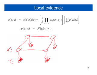
![Boltzmann distribution
• Prob distribution in terms of clique potentials
1
p(x|θ) = ψc (xc |θ c )
Z(θ)
c∈C
• In terms of energy functions
ψc (xc ) = exp[−Hc (xc )]
log p(x) = −[ Hc (xc ) + log Z]
c∈C
6](https://image.slidesharecdn.com/denoise-1302622884-phpapp02/85/Image-denoising-6-320.jpg)
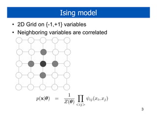
![Ising model
• 2D Grid on {-1,+1} variables
• Neighboring variables are correlated
Wij −Wij
Hij =
−Wij Wij
W > 0: ferro magnet
W < 0: anti ferro magnet (frustrated)
H(x) = −xT Wx = − Wij xi xj
<ij>
1
p(x|θ ) = exp[−βH(x|θ )]
Z(θ )
β=1/T = inverse temperature 7](https://image.slidesharecdn.com/denoise-1302622884-phpapp02/85/Image-denoising-7-320.jpg)
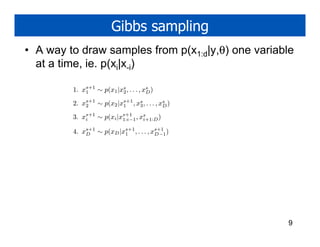
![Gibbs sampling in an MRF
• Full conditional depends only on Markov blanket
p(xi = ℓ, x−i )
p(Xi = ℓ|x−i ) = ′
ℓ′ p(Xi = ℓ , x−i )
(1/Z)[ j∈Ni ψij (Xi = ℓ, xj )][ <jk>:j,k∈Fi ψjk (xj , xk )]
=
(1/Z) ℓ′ [ j∈Ni ψij (Xi = ℓ′ , xj )][ <j,k>:j,k∈Fi ψjk (xj , xk )]
j∈Ni ψij (Xi = ℓ, xj )
=
ℓ′ j∈Ni ψij (Xi = ℓ′ , xj )
11](https://image.slidesharecdn.com/denoise-1302622884-phpapp02/85/Image-denoising-11-320.jpg)
![Gibbs sampling in an Ising model
• Let ψ(xi,xj) = exp(W xi xj), xi = +1,-1.
j∈Ni ψij (Xi = +1, xj )
p(Xi = +1|x−i ) =
j∈Ni ψij (Xi = +1, xj ) + j∈Ni ψij (Xi = −1, xj )
exp[J j∈Ni xj ]
=
exp[J j∈Ni xj ] + exp[−J j∈Ni xj ]
exp[Jwi ]
=
exp[Jwi ] + exp[−Jwi ]
= σ(2J wi )
wi = xj
j∈Ni
σ(u) = 1/(1 + e−u )
12](https://image.slidesharecdn.com/denoise-1302622884-phpapp02/85/Image-denoising-12-320.jpg)
![Adding in local evidence
• Final form is
exp[J wi ]φi (+1, yi )
p(Xi = +1|x−i , y) =
exp[Jwi ]φi (+1, yi ) + exp[−Jwi ]φi (−1, yi )
Run demo
13](https://image.slidesharecdn.com/denoise-1302622884-phpapp02/85/Image-denoising-13-320.jpg)
![Gibbs sampling for DAGs
• The Markov blanket of a node is the set that
renders it independent of the rest of the graph.
• This is the parents, children and co-parents.
p(Xi , X−i )
p(Xi |X−i ) =
x p(Xi , X−i )
p(Xi , U1:n , Y1:m , Z1:m , R)
=
x p(x, U1:n , Y1:m , Z1:m , R)
p(Xi |U1:n )[ j p(Yj |Xi , Zj )]P (U1:n , Z1:m , R)
=
x p(Xi = x|U1:n )[ j p(Yj |Xi = x, Zj )]P (U1:n , Z1:m , R)
p(Xi |U1:n )[ j p(Yj |Xi , Zj )]
=
x p(Xi = x|U1:n )[ j p(Yj |Xi = x, Zj )]
p(Xi |X−i ) ∝ p(Xi |P a(Xi )) p(Yj |P a(Yj )
Yj ∈ch(Xi )
14](https://image.slidesharecdn.com/denoise-1302622884-phpapp02/85/Image-denoising-14-320.jpg)
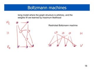

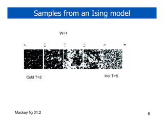
1. Gibbs sampling is a technique for drawing samples from probability distributions by iteratively sampling each variable conditioned on the current values of the other variables. It can be used to sample from Markov random fields and Bayesian networks. 2. An Ising model is a Markov random field with binary variables on a grid that are correlated with their neighbors. Gibbs sampling in an Ising model samples each variable based on its neighbors' current values. 3. Boltzmann machines generalize the Ising model to arbitrary graph structures between variables. Restricted Boltzmann machines and Hopfield networks are specific types of Boltzmann machines.