Sparse Coding and Dictionary Learning
                              for Image Analysis
              Part III: Optimization for Sparse Coding and Dictionary Learning


           Francis Bach, Julien Mairal, Jean Ponce and Guillermo Sapiro


                      CVPR’10 tutorial, San Francisco, 14th June 2010


Francis Bach, Julien Mairal, Jean Ponce and Guillermo Sapiro   Part III: Optimization   1/52
The Sparse Decomposition Problem

                                     1
                        minp           ||x − Dα||2
                                                 2                     +           λψ(α)
                       α∈R           2
                                                                             sparsity-inducing
                                      data fitting term                        regularization

   ψ induces sparsity in α. It can be
                                                               △
           the ℓ0 “pseudo-norm”. ||α||0 = #{i s.t. α[i ] = 0} (NP-hard)
                                            △       p
           the ℓ1 norm. ||α||1 =                    i =1 |α[i ]|     (convex)
           ...
   This is a selection problem.


Francis Bach, Julien Mairal, Jean Ponce and Guillermo Sapiro       Part III: Optimization        2/52
Finding your way in the sparse coding literature. . .
   . . . is not easy. The literature is vast, redundant, sometimes
   confusing and many papers are claiming victory. . .

   The main class of methods are
       greedy procedures [Mallat and Zhang, 1993], [Weisberg, 1980]
       homotopy [Osborne et al., 2000], [Efron et al., 2004],
       [Markowitz, 1956]
       soft-thresholding based methods [Fu, 1998], [Daubechies et al.,
       2004], [Friedman et al., 2007], [Nesterov, 2007], [Beck and
       Teboulle, 2009], . . .
       reweighted-ℓ2 methods [Daubechies et al., 2009],. . .
       active-set methods [Roth and Fischer, 2008].
       ...


Francis Bach, Julien Mairal, Jean Ponce and Guillermo Sapiro   Part III: Optimization   3/52
Matching Pursuit                                                                             α = (0, 0, 0)
                               y
                                          d2


                                                               d1

                                                  z                        r=x


                                                                                              d3


                                                                                             x
Francis Bach, Julien Mairal, Jean Ponce and Guillermo Sapiro        Part III: Optimization              4/52
Matching Pursuit                                                                             α = (0, 0, 0)
                               y
                                          d2


                                                               d1

                                                  z                             r


                                                                                              d3
                                                                      < r, d3 > d3
                                                                                             x
Francis Bach, Julien Mairal, Jean Ponce and Guillermo Sapiro        Part III: Optimization              5/52
Matching Pursuit                                                                             α = (0, 0, 0)
                               y
                                          d2


                                                               d1

                                                  z                             r
                                                                                    r− < r, d3 > d3

                                                                                              d3


                                                                                             x
Francis Bach, Julien Mairal, Jean Ponce and Guillermo Sapiro        Part III: Optimization              6/52
Matching Pursuit                                                                             α = (0, 0, 0.75)
                                y
                                          d2


                                                               d1

                                                  z
                            r

                                                                                                 d3


                                                                                                 x
Francis Bach, Julien Mairal, Jean Ponce and Guillermo Sapiro        Part III: Optimization                 7/52
Matching Pursuit                                                                             α = (0, 0, 0.75)
                                y
                                          d2


                                                               d1

                                                  z
                            r

                                                                                                 d3


                                                                                                 x
Francis Bach, Julien Mairal, Jean Ponce and Guillermo Sapiro        Part III: Optimization                 8/52
Matching Pursuit                                                                             α = (0, 0, 0.75)
                                y
                                          d2


                                                               d1

                                                  z
                            r

                                                                                                 d3


                                                                                                 x
Francis Bach, Julien Mairal, Jean Ponce and Guillermo Sapiro        Part III: Optimization                 9/52
Matching Pursuit                                                                      α = (0, 0.24, 0.75)
                               y
                                          d2


                                                               d1

                                                  z


                                                                                             d3
                        r

                                                                                             x
Francis Bach, Julien Mairal, Jean Ponce and Guillermo Sapiro        Part III: Optimization             10/52
Matching Pursuit                                                                      α = (0, 0.24, 0.75)
                               y
                                          d2


                                                               d1

                                                  z


                                                                                             d3
                        r

                                                                                             x
Francis Bach, Julien Mairal, Jean Ponce and Guillermo Sapiro        Part III: Optimization             11/52
Matching Pursuit                                                                      α = (0, 0.24, 0.75)
                               y
                                          d2


                                                               d1

                                                  z


                                                                                             d3
                        r

                                                                                             x
Francis Bach, Julien Mairal, Jean Ponce and Guillermo Sapiro        Part III: Optimization             12/52
Matching Pursuit                                                                      α = (0, 0.24, 0.65)
                               y
                                          d2


                                                               d1

                                                  z


                                                                                             d3
                               r

                                                                                             x
Francis Bach, Julien Mairal, Jean Ponce and Guillermo Sapiro        Part III: Optimization             13/52
Matching Pursuit

                                   min || x − Dα ||2 s.t. ||α||0 ≤ L
                                                   2
                                  α∈Rp
                                                     r


     1: α←0
     2: r ← x (residual).
     3: while ||α||0 < L do
     4:   Select the atom with maximum correlation with the residual

                                                     ˆ ← arg max |dT r|
                                                     ı             i
                                                               i =1,...,p

     5:      Update the residual and the coefficients
                                                                 T
                                                  α[ˆ] ← α[ˆ] + dˆ r
                                                    ı      ı     ı
                                                                   T
                                                         r ← r − (dˆ r)dˆ
                                                                   ı    ı

     6:   end while
Francis Bach, Julien Mairal, Jean Ponce and Guillermo Sapiro      Part III: Optimization   14/52
Orthogonal Matching Pursuit                                                                  α = (0, 0, 0)
            y                                                                                      Γ=∅
                 d2


                                                               d1

                                                  z                             x


                                                                                              d3


                                                                                             x
Francis Bach, Julien Mairal, Jean Ponce and Guillermo Sapiro        Part III: Optimization              15/52
Orthogonal Matching Pursuit                                                                  α = (0, 0, 0.75)
            y                                                                                       Γ = {3}
                 d2


                                           π2                  d1

                                                  z                             x
                                                                                    r

                                     π1
                                                                                                 d3
                                                                                 π3

                                                                                                 x
Francis Bach, Julien Mairal, Jean Ponce and Guillermo Sapiro        Part III: Optimization                 16/52
Orthogonal Matching Pursuit                                                           α = (0, 0.29, 0.63)
            y                                                                                 Γ = {3, 2}
                 d2


                                                               d1

                                                  z                        x
                                                                       π 32 r

                                                                           π 31              d3


                                                                                             x
Francis Bach, Julien Mairal, Jean Ponce and Guillermo Sapiro        Part III: Optimization             17/52
Orthogonal Matching Pursuit

                                    min ||x − Dα||2 s.t. ||α||0 ≤ L
                                                  2
                                   α∈Rp


     1: Γ = ∅.
     2: for iter = 1, . . . , L do
     3:   Select the atom which most reduces the objective

                                      ˆ ← arg min min ||x − DΓ∪{i } α′ ||2
                                      ı             ′                    2
                                                i ∈ΓC          α

     4:      Update the active set: Γ ← Γ ∪ {ˆ}.
                                              ı
     5:      Update the residual (orthogonal projection)
                                            r ← (I − DΓ (DT DΓ )−1 DT )x.
                                                          Γ         Γ

     6:      Update the coefficients
                                                 αΓ ← (DT DΓ )−1 DT x.
                                                        Γ         Γ

     7:   end for
Francis Bach, Julien Mairal, Jean Ponce and Guillermo Sapiro       Part III: Optimization   18/52
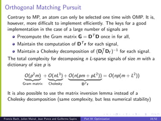
Orthogonal Matching Pursuit
   Contrary to MP, an atom can only be selected one time with OMP. It is,
   however, more difficult to implement efficiently. The keys for a good
   implementation in the case of a large number of signals are
           Precompute the Gram matrix G = DT D once in for all,
           Maintain the computation of DT r for each signal,
           Maintain a Cholesky decomposition of (DΓ DΓ )−1 for each signal.
                                                  T

   The total complexity for decomposing n L-sparse signals of size m with a
   dictionary of size p is

                O(p 2 m) + O(nL3 ) + O(n(pm + pL2 )) = O(np(m + L2 ))
               Gram matrix          Cholesky                   DT r

   It is also possible to use the matrix inversion lemma instead of a
   Cholesky decomposition (same complexity, but less numerical stability)


Francis Bach, Julien Mairal, Jean Ponce and Guillermo Sapiro    Part III: Optimization   19/52
Example with the software SPAMS
   Software available at http://www.di.ens.fr/willow/SPAMS/

         >>    I=double(imread(’data/lena.eps’))/255;
         >>    %extract all patches of I
         >>    X=im2col(I,[8 8],’sliding’);
         >>    %load a dictionary of size 64 x 256
         >>    D=load(’dict.mat’);
         >>
         >>    %set the sparsity parameter L to 10
         >>    param.L=10;
         >>    alpha=mexOMP(X,D,param);


   On a 8-cores 2.83Ghz machine: 230000 signals processed per second!


Francis Bach, Julien Mairal, Jean Ponce and Guillermo Sapiro   Part III: Optimization   20/52
Optimality conditions of the Lasso
Nonsmooth optimization

   Directional derivatives and subgradients are useful tools for studying
   ℓ1 -decomposition problems:
                                                 1
                                        min        ||x − Dα||2 + λ||α||1
                                                             2
                                       α∈Rp      2

   In this tutorial, we use the directional derivatives to derive simple
   optimality conditions of the Lasso.

   For more information on convex analysis and nonsmooth optimization,
   see the following books: [Boyd and Vandenberghe, 2004], [Nocedal and
   Wright, 2006], [Borwein and Lewis, 2006], [Bonnans et al., 2006],
   [Bertsekas, 1999].


Francis Bach, Julien Mairal, Jean Ponce and Guillermo Sapiro   Part III: Optimization   21/52
Optimality conditions of the Lasso
Directional derivatives

           Directional derivative in the direction u at α:
                                                                 f (α + tu) − f (α)
                                     ∇f (α, u) = lim+
                                                          t→0            t
           Main idea: in non smooth situations, one may need to look at all
           directions u and not simply p independent ones!
           Proposition 1: if f is differentiable in α, ∇f (α, u) = ∇f (α)T u.
           Proposition 2: α is optimal iff for all u in Rp , ∇f (α, u) ≥ 0.


Francis Bach, Julien Mairal, Jean Ponce and Guillermo Sapiro    Part III: Optimization   22/52
Optimality conditions of the Lasso

                                                 1
                                        minp       ||x − Dα||2 + λ||α||1
                                                             2
                                       α∈R       2
   α⋆    is optimal iff for all u in Rp , ∇f (α, u) ≥ 0—that is,

        −uT DT (x − Dα⋆ ) + λ                                  sign(α⋆ [i ])u[i ] + λ                      |ui | ≥ 0,
                                               i ,α⋆ [i ]=0                                 i ,α⋆ [i ]=0

   which is equivalent to the following conditions:

                                     |dT (x − Dα⋆ )| ≤ λ
                                       i                                                           if α⋆ [i ] = 0
     ∀i = 1, . . . , p,
                                      dT (x − Dα⋆ ) = λ sign(α⋆ [i ])
                                       i                                                           if α⋆ [i ] = 0


Francis Bach, Julien Mairal, Jean Ponce and Guillermo Sapiro       Part III: Optimization                               23/52
Homotopy
           A homotopy method provides a set of solutions indexed by a
           parameter.
           The regularization path (λ, α⋆ (λ)) for instance!!
           It can be useful when the path has some “nice” properties
           (piecewise linear, piecewise quadratic).
           LARS [Efron et al., 2004] starts from a trivial solution, and follows
           the regularization path of the Lasso, which is is piecewise linear.


Francis Bach, Julien Mairal, Jean Ponce and Guillermo Sapiro   Part III: Optimization   24/52
Homotopy, LARS
[Osborne et al., 2000], [Efron et al., 2004]

                                     |diT (x − Dα⋆ )| ≤ λ                               if α⋆ [i ] = 0
     ∀i = 1, . . . , p,
                                      diT (x − Dα⋆ ) = λ sign(α⋆ [i ])                  if α⋆ [i ] = 0
                                                                                                         (1)
   The regularization path is piecewise linear:

                    DT (x − DΓ α⋆ ) = λ sign(α⋆ )
                     Γ          Γ             Γ
                    α⋆ (λ) = (DT DΓ )−1 (DT x − λ sign(α⋆ )) = A + λB
                     Γ         Γ          Γ             Γ

   A simple interpretation of LARS
           Start from the trivial solution (λ = ||DT x||∞ , α⋆ (λ) = 0).
           Maintain the computations of |dT (x − Dα⋆ (λ))| for all i .
                                          i
           Maintain the computation of the current direction B.
           Follow the path by reducing λ until the next kink.


Francis Bach, Julien Mairal, Jean Ponce and Guillermo Sapiro   Part III: Optimization                    25/52
Example with the software SPAMS
http://www.di.ens.fr/willow/SPAMS/


         >>    I=double(imread(’data/lena.eps’))/255;
         >>    %extract all patches of I
         >>    X=normalize(im2col(I,[8 8],’sliding’));
         >>    %load a dictionary of size 64 x 256
         >>    D=load(’dict.mat’);
         >>
         >>    %set the sparsity parameter lambda to 0.15
         >>    param.lambda=0.15;
         >>    alpha=mexLasso(X,D,param);


   On a 8-cores 2.83Ghz machine: 77000 signals processed per second!
   Note that it can also solve constrained version of the problem. The
   complexity is more or less the same as OMP and uses the same tricks
   (Cholesky decomposition).
Francis Bach, Julien Mairal, Jean Ponce and Guillermo Sapiro   Part III: Optimization   26/52
Coordinate Descent
           Coordinate descent + nonsmooth objective: WARNING: not
           convergent in general
           Here, the problem is equivalent to a convex smooth optimization
           problem with separable constraints
                     1
            min        ||x − D+ α+ + D− α− ||2 + λα+ 1 + λαT 1 s.t. α− , α+ ≥ 0.
                                             2
                                                   T
                                                           −
           α+ ,α−    2
           For this specific problem, coordinate descent is convergent.
           Supposing ||di ||2 = 1, updating the coordinate i :
                                          1
                           α[i ] ← arg min || x −                    α[j]dj −βdi ||2 + λ|β|
                                                                                   2
                                      β   2
                                                               j=i

                                                           r
                                   ←    sign(di r)(|di r| − λ)+
                                              T      T


           ⇒ soft-thresholding!
Francis Bach, Julien Mairal, Jean Ponce and Guillermo Sapiro   Part III: Optimization         27/52
Example with the software SPAMS
http://www.di.ens.fr/willow/SPAMS/


         >>    I=double(imread(’data/lena.eps’))/255;
         >>    %extract all patches of I
         >>    X=normalize(im2col(I,[8 8],’sliding’));
         >>    %load a dictionary of size 64 x 256
         >>    D=load(’dict.mat’);
         >>
         >>    %set the sparsity parameter lambda to 0.15
         >>    param.lambda=0.15;
         >>    param.tol=1e-2;
         >>    param.itermax=200;
         >>    alpha=mexCD(X,D,param);


   On a 8-cores 2.83Ghz machine: 93000 signals processed per second!

Francis Bach, Julien Mairal, Jean Ponce and Guillermo Sapiro   Part III: Optimization   28/52
first-order/proximal methods

                                               min f (α) + λψ(α)
                                              α∈Rp


           f is strictly convex and continuously differentiable with a Lipshitz
           gradient.
           Generalize the idea of gradient descent
                                                       L
           αk+1 ← arg min f (αk )+∇f (αk )T (α − αk )+ ||α − αk ||2 +λψ(α)
                                                                  2
                    α∈R                                2
                            1            1               λ
                ← arg min ||α − (αk − ∇f (αk ))||2 + ψ(α)
                                                     2
                     α∈R 2               L               L

           When λ = 0, this is equivalent to a classical gradient descent step.


Francis Bach, Julien Mairal, Jean Ponce and Guillermo Sapiro   Part III: Optimization   29/52
first-order/proximal methods
           They require solving efficiently the proximal operator
                                                       1             2
                                              minp       u−α         2   + λψ(α)
                                             α∈R       2
           For the ℓ1 -norm, this amounts to a soft-thresholding:

                                           α⋆ [i ] = sign(u[i ])(u[i ] − λ)+ .

           There exists accelerated versions based on Nesterov optimal
           first-order method (gradient method with “extrapolation”) [Beck
           and Teboulle, 2009, Nesterov, 2007, 1983]
           suited for large-scale experiments.


Francis Bach, Julien Mairal, Jean Ponce and Guillermo Sapiro   Part III: Optimization   30/52
Optimization for Grouped Sparsity
   The formulation:
                                       1                  2
                            min          x − Dα           2    +      λ           αg    q
                            α∈Rp       2
                                                                          g ∈G
                                      data fitting term
                                                                   group-sparsity-inducing
                                                                       regularization

    The main class of algorithms for solving grouped-sparsity problems are
           Greedy approaches
           Block-coordinate descent
           Proximal methods


Francis Bach, Julien Mairal, Jean Ponce and Guillermo Sapiro   Part III: Optimization        31/52
Optimization for Grouped Sparsity
   The proximal operator:
                                              1                2
                                     minp       u−α            2   +λ              αg       q
                                    α∈R       2
                                                                          g ∈G

    For q = 2,
                                              ug
                                  ⋆
                                 αg =              ( ug        2   − λ)+ , ∀g ∈ G
                                              ug 2
    For q = ∞,
                                    α⋆ = ug − Π
                                     g                     . 1 ≤λ [ug ],         ∀g ∈ G
    These formula generalize soft-thrsholding to groups of variables. They
   are used in block-coordinate descent and proximal algorithms.


Francis Bach, Julien Mairal, Jean Ponce and Guillermo Sapiro       Part III: Optimization       32/52
Reweighted ℓ2
   Let us start from something simple

                                              a2 − 2ab + b2 ≥ 0.

    Then
                                   1 a2
                           a≤           +b                with equality iff a = b
                                   2 b
    and
                                                                    p
                                                   1                     α[j]2
                                    ||α||1 = min                               + ηj .
                                             ηj ≥0 2                      ηj
                                                                   j=1

    The formulation becomes
                                                                            p
                                    1                          2     λ           α[j]2
                             min      x − Dα                   2   +                   + ηj .
                            α,ηj ≥ε 2                                2            ηj
                                                                          j=1


Francis Bach, Julien Mairal, Jean Ponce and Guillermo Sapiro        Part III: Optimization      33/52
Summary so far
           Greedy methods directly address the NP-hard ℓ0 -decomposition
           problem.
           Homotopy methods can be extremely efficient for small or
           medium-sized problems, or when the solution is very sparse.
           Coordinate descent provides in general quickly a solution with a
           small/medium precision, but gets slower when there is a lot of
           correlation in the dictionary.
           First order methods are very attractive in the large scale setting.
           Other good alternatives exists, active-set, reweighted ℓ2 methods,
           stochastic variants, variants of OMP,. . .


Francis Bach, Julien Mairal, Jean Ponce and Guillermo Sapiro   Part III: Optimization   34/52
Optimization for Dictionary Learning

                                          n
                                                1
                            min                   ||xi − Dαi ||2 + λ||αi ||1
                                                               2
                         α∈R  p×n               2
                          D∈C           i=1
              △
         C = {D ∈ Rm×p s.t. ∀j = 1, . . . , p, ||dj ||2 ≤ 1}.


           Classical optimization alternates between D and α.
           Good results, but very slow!


Francis Bach, Julien Mairal, Jean Ponce and Guillermo Sapiro   Part III: Optimization   35/52
Optimization for Dictionary Learning
[Mairal, Bach, Ponce, and Sapiro, 2009a]

   Classical formulation of dictionary learning
                                                                      n
                                                                 1
                                     min fn (D) = min                       l (xi , D),
                                     D∈C                   D∈C   n
                                                                     i =1

   where
                                        △     1
                               l (x, D) = minp ||x − Dα||2 + λ||α||1 .
                                                         2
                                          α∈R 2

   Which formulation are we interested in?
                                                                                     n
                                                      1
                      min f (D) = Ex [l (x, D)] ≈ lim                                     l (xi , D)
                      D∈C                        n→+∞ n
                                                                                   i =1

   [Bottou and Bousquet, 2008]: Online learning can
           handle potentially infinite or dynamic datasets,
           be dramatically faster than batch algorithms.
Francis Bach, Julien Mairal, Jean Ponce and Guillermo Sapiro     Part III: Optimization                36/52
Optimization for Dictionary Learning
   Require: D0 ∈ Rm×p (initial dictionary); λ ∈ R
    1: A0 = 0, B0 = 0.
    2: for t=1,. . . ,T do
    3: Draw xt
    4: Sparse Coding

                                             1
                                 αt ← arg min ||xt − Dt−1 α||2 + λ||α||1 ,
                                                             2
                                       α∈Rp 2

     5:     Aggregate sufficient statistics
            At ← At−1 + αt αT , Bt ← Bt−1 + xt αT
                              t                    t
     6:     Dictionary Update (block-coordinate descent)
                                                        t
                                                   1           1
                           Dt ← arg min                          ||xi − Dαi ||2 + λ||αi ||1 .
                                                                              2
                                         D∈C       t           2
                                                       i =1

     7:   end for
Francis Bach, Julien Mairal, Jean Ponce and Guillermo Sapiro    Part III: Optimization          37/52
Optimization for Dictionary Learning
   Which guarantees do we have?
   Under a few reasonable assumptions,
                                     ˆ
       we build a surrogate function ft of the expected cost f verifying

                                                   ˆ
                                               lim ft (Dt ) − f (Dt ) = 0,
                                             t→+∞

           Dt is asymptotically close to a stationary point.

   Extensions (all implemented in SPAMS)
           non-negative matrix decompositions.
           sparse PCA (sparse dictionaries).
           fused-lasso regularizations (piecewise constant dictionaries)


Francis Bach, Julien Mairal, Jean Ponce and Guillermo Sapiro   Part III: Optimization   38/52
Optimization for Dictionary Learning
Experimental results, batch vs online


                                             m = 8 × 8, p = 256
Francis Bach, Julien Mairal, Jean Ponce and Guillermo Sapiro   Part III: Optimization   39/52
Optimization for Dictionary Learning
Experimental results, batch vs online


                                       m = 12 × 12 × 3, p = 512
Francis Bach, Julien Mairal, Jean Ponce and Guillermo Sapiro   Part III: Optimization   40/52
Optimization for Dictionary Learning
Inpainting a 12-Mpixel photograph


Francis Bach, Julien Mairal, Jean Ponce and Guillermo Sapiro   Part III: Optimization   41/52
Optimization for Dictionary Learning
Inpainting a 12-Mpixel photograph


Francis Bach, Julien Mairal, Jean Ponce and Guillermo Sapiro   Part III: Optimization   42/52
Optimization for Dictionary Learning
Inpainting a 12-Mpixel photograph


Francis Bach, Julien Mairal, Jean Ponce and Guillermo Sapiro   Part III: Optimization   43/52
Optimization for Dictionary Learning
Inpainting a 12-Mpixel photograph


Francis Bach, Julien Mairal, Jean Ponce and Guillermo Sapiro   Part III: Optimization   44/52
Extension to NMF and sparse PCA
[Mairal, Bach, Ponce, and Sapiro, 2009b]

   NMF extension
                                    n
                                         1
                         min               ||xi − Dαi ||2 s.t. αi ≥ 0,
                                                        2                               D ≥ 0.
                      α∈Rp×n             2
                       D∈C i =1


   SPCA extension
                                               n
                                                    1
                                   min                ||xi − Dαi ||2 + λ||α1 ||1
                                                                   2
                                 α∈Rp×n             2
                                  D∈C ′      i =1

                           △
                      C ′ = {D ∈ Rm×p s.t. ∀j ||dj ||2 + γ||dj ||1 ≤ 1}.
                                                     2


Francis Bach, Julien Mairal, Jean Ponce and Guillermo Sapiro   Part III: Optimization            45/52
Extension to NMF and sparse PCA
Faces: Extended Yale Database B


                 (a) PCA                               (b) NNMF                         (c) DL


Francis Bach, Julien Mairal, Jean Ponce and Guillermo Sapiro   Part III: Optimization            46/52
Extension to NMF and sparse PCA
Faces: Extended Yale Database B


         (d) SPCA, τ = 70%                       (e) SPCA, τ = 30%                      (f) SPCA, τ = 10%


Francis Bach, Julien Mairal, Jean Ponce and Guillermo Sapiro   Part III: Optimization                       47/52
Extension to NMF and sparse PCA
Natural Patches


                 (a) PCA                               (b) NNMF                         (c) DL


Francis Bach, Julien Mairal, Jean Ponce and Guillermo Sapiro   Part III: Optimization            48/52
Extension to NMF and sparse PCA
Natural Patches


         (d) SPCA, τ = 70%                       (e) SPCA, τ = 30%                      (f) SPCA, τ = 10%


Francis Bach, Julien Mairal, Jean Ponce and Guillermo Sapiro   Part III: Optimization                       49/52
References I
   A. Beck and M. Teboulle. A fast iterative shrinkage-thresholding algorithm for linear
      inverse problems. SIAM Journal on Imaging Sciences, 2(1):183–202, 2009.
   D. P. Bertsekas. Nonlinear programming. Athena Scientific Belmont, Mass, 1999.
   J.F. Bonnans, J.C. Gilbert, C. Lemarechal, and C.A. Sagastizabal. Numerical
      optimization: theoretical and practical aspects. Springer-Verlag New York Inc,
      2006.
   J. M. Borwein and A. S. Lewis. Convex analysis and nonlinear optimization: Theory
      and examples. Springer, 2006.
   L. Bottou and O. Bousquet. The trade-offs of large scale learning. In J.C. Platt,
      D. Koller, Y. Singer, and S. Roweis, editors, Advances in Neural Information
      Processing Systems, volume 20, pages 161–168. MIT Press, Cambridge, MA, 2008.
   S. P. Boyd and L. Vandenberghe. Convex Optimization. Cambridge University Press,
      2004.
   I. Daubechies, M. Defrise, and C. De Mol. An iterative thresholding algorithm for
      linear inverse problems with a sparsity constraint. Comm. Pure Appl. Math, 57:
      1413–1457, 2004.


Francis Bach, Julien Mairal, Jean Ponce and Guillermo Sapiro   Part III: Optimization   50/52
References II
   I. Daubechies, R. DeVore, M. Fornasier, and S. Gunturk. Iteratively re-weighted least
      squares minimization for sparse recovery. Commun. Pure Appl. Math, 2009.
   B. Efron, T. Hastie, I. Johnstone, and R. Tibshirani. Least angle regression. Annals of
      statistics, 32(2):407–499, 2004.
   J. Friedman, T. Hastie, H. H¨lfling, and R. Tibshirani. Pathwise coordinate
                                o
      optimization. Annals of statistics, 1(2):302–332, 2007.
   W. J. Fu. Penalized regressions: The bridge versus the Lasso. Journal of
     computational and graphical statistics, 7:397–416, 1998.
   J. Mairal, F. Bach, J. Ponce, and G. Sapiro. Online dictionary learning for sparse
      coding. In Proceedings of the International Conference on Machine Learning
      (ICML), 2009a.
   J. Mairal, F. Bach, J. Ponce, and G. Sapiro. Online learning for matrix factorization
      and sparse coding. ArXiv:0908.0050v1, 2009b. submitted.
   S. Mallat and Z. Zhang. Matching pursuit in a time-frequency dictionary. IEEE
      Transactions on Signal Processing, 41(12):3397–3415, 1993.
   H. M. Markowitz. The optimization of a quadratic function subject to linear
      constraints. Naval Research Logistics Quarterly, 3:111–133, 1956.


Francis Bach, Julien Mairal, Jean Ponce and Guillermo Sapiro   Part III: Optimization   51/52
References III
   Y. Nesterov. Gradient methods for minimizing composite objective function.
      Technical report, CORE, 2007.
   Y. Nesterov. A method for solving a convex programming problem with convergence
      rate O(1/k 2 ). Soviet Math. Dokl., 27:372–376, 1983.
   J. Nocedal and SJ Wright. Numerical Optimization. Springer: New York, 2006. 2nd
      Edition.
   M. R. Osborne, B. Presnell, and B. A. Turlach. On the Lasso and its dual. Journal of
     Computational and Graphical Statistics, 9(2):319–37, 2000.
   V. Roth and B. Fischer. The group-lasso for generalized linear models: uniqueness of
      solutions and efficient algorithms. In Proceedings of the International Conference
      on Machine Learning (ICML), 2008.
   S. Weisberg. Applied Linear Regression. Wiley, New York, 1980.


Francis Bach, Julien Mairal, Jean Ponce and Guillermo Sapiro   Part III: Optimization   52/52

CVPR2010: Sparse Coding and Dictionary Learning for Image Analysis: Part 3: Optimization Techniques for Sparse Coding

  • 1.
    Sparse Coding andDictionary Learning for Image Analysis Part III: Optimization for Sparse Coding and Dictionary Learning Francis Bach, Julien Mairal, Jean Ponce and Guillermo Sapiro CVPR’10 tutorial, San Francisco, 14th June 2010 Francis Bach, Julien Mairal, Jean Ponce and Guillermo Sapiro Part III: Optimization 1/52
  • 2.
    The Sparse DecompositionProblem 1 minp ||x − Dα||2 2 + λψ(α) α∈R 2 sparsity-inducing data fitting term regularization ψ induces sparsity in α. It can be △ the ℓ0 “pseudo-norm”. ||α||0 = #{i s.t. α[i ] = 0} (NP-hard) △ p the ℓ1 norm. ||α||1 = i =1 |α[i ]| (convex) ... This is a selection problem. Francis Bach, Julien Mairal, Jean Ponce and Guillermo Sapiro Part III: Optimization 2/52
  • 3.
    Finding your wayin the sparse coding literature. . . . . . is not easy. The literature is vast, redundant, sometimes confusing and many papers are claiming victory. . . The main class of methods are greedy procedures [Mallat and Zhang, 1993], [Weisberg, 1980] homotopy [Osborne et al., 2000], [Efron et al., 2004], [Markowitz, 1956] soft-thresholding based methods [Fu, 1998], [Daubechies et al., 2004], [Friedman et al., 2007], [Nesterov, 2007], [Beck and Teboulle, 2009], . . . reweighted-ℓ2 methods [Daubechies et al., 2009],. . . active-set methods [Roth and Fischer, 2008]. ... Francis Bach, Julien Mairal, Jean Ponce and Guillermo Sapiro Part III: Optimization 3/52
  • 4.
    Matching Pursuit α = (0, 0, 0) y d2 d1 z r=x d3 x Francis Bach, Julien Mairal, Jean Ponce and Guillermo Sapiro Part III: Optimization 4/52
  • 5.
    Matching Pursuit α = (0, 0, 0) y d2 d1 z r d3 < r, d3 > d3 x Francis Bach, Julien Mairal, Jean Ponce and Guillermo Sapiro Part III: Optimization 5/52
  • 6.
    Matching Pursuit α = (0, 0, 0) y d2 d1 z r r− < r, d3 > d3 d3 x Francis Bach, Julien Mairal, Jean Ponce and Guillermo Sapiro Part III: Optimization 6/52
  • 7.
    Matching Pursuit α = (0, 0, 0.75) y d2 d1 z r d3 x Francis Bach, Julien Mairal, Jean Ponce and Guillermo Sapiro Part III: Optimization 7/52
  • 8.
    Matching Pursuit α = (0, 0, 0.75) y d2 d1 z r d3 x Francis Bach, Julien Mairal, Jean Ponce and Guillermo Sapiro Part III: Optimization 8/52
  • 9.
    Matching Pursuit α = (0, 0, 0.75) y d2 d1 z r d3 x Francis Bach, Julien Mairal, Jean Ponce and Guillermo Sapiro Part III: Optimization 9/52
  • 10.
    Matching Pursuit α = (0, 0.24, 0.75) y d2 d1 z d3 r x Francis Bach, Julien Mairal, Jean Ponce and Guillermo Sapiro Part III: Optimization 10/52
  • 11.
    Matching Pursuit α = (0, 0.24, 0.75) y d2 d1 z d3 r x Francis Bach, Julien Mairal, Jean Ponce and Guillermo Sapiro Part III: Optimization 11/52
  • 12.
    Matching Pursuit α = (0, 0.24, 0.75) y d2 d1 z d3 r x Francis Bach, Julien Mairal, Jean Ponce and Guillermo Sapiro Part III: Optimization 12/52
  • 13.
    Matching Pursuit α = (0, 0.24, 0.65) y d2 d1 z d3 r x Francis Bach, Julien Mairal, Jean Ponce and Guillermo Sapiro Part III: Optimization 13/52
  • 14.
    Matching Pursuit min || x − Dα ||2 s.t. ||α||0 ≤ L 2 α∈Rp r 1: α←0 2: r ← x (residual). 3: while ||α||0 < L do 4: Select the atom with maximum correlation with the residual ˆ ← arg max |dT r| ı i i =1,...,p 5: Update the residual and the coefficients T α[ˆ] ← α[ˆ] + dˆ r ı ı ı T r ← r − (dˆ r)dˆ ı ı 6: end while Francis Bach, Julien Mairal, Jean Ponce and Guillermo Sapiro Part III: Optimization 14/52
  • 15.
    Orthogonal Matching Pursuit α = (0, 0, 0) y Γ=∅ d2 d1 z x d3 x Francis Bach, Julien Mairal, Jean Ponce and Guillermo Sapiro Part III: Optimization 15/52
  • 16.
    Orthogonal Matching Pursuit α = (0, 0, 0.75) y Γ = {3} d2 π2 d1 z x r π1 d3 π3 x Francis Bach, Julien Mairal, Jean Ponce and Guillermo Sapiro Part III: Optimization 16/52
  • 17.
    Orthogonal Matching Pursuit α = (0, 0.29, 0.63) y Γ = {3, 2} d2 d1 z x π 32 r π 31 d3 x Francis Bach, Julien Mairal, Jean Ponce and Guillermo Sapiro Part III: Optimization 17/52
  • 18.
    Orthogonal Matching Pursuit min ||x − Dα||2 s.t. ||α||0 ≤ L 2 α∈Rp 1: Γ = ∅. 2: for iter = 1, . . . , L do 3: Select the atom which most reduces the objective ˆ ← arg min min ||x − DΓ∪{i } α′ ||2 ı ′ 2 i ∈ΓC α 4: Update the active set: Γ ← Γ ∪ {ˆ}. ı 5: Update the residual (orthogonal projection) r ← (I − DΓ (DT DΓ )−1 DT )x. Γ Γ 6: Update the coefficients αΓ ← (DT DΓ )−1 DT x. Γ Γ 7: end for Francis Bach, Julien Mairal, Jean Ponce and Guillermo Sapiro Part III: Optimization 18/52
  • 19.
    Orthogonal Matching Pursuit Contrary to MP, an atom can only be selected one time with OMP. It is, however, more difficult to implement efficiently. The keys for a good implementation in the case of a large number of signals are Precompute the Gram matrix G = DT D once in for all, Maintain the computation of DT r for each signal, Maintain a Cholesky decomposition of (DΓ DΓ )−1 for each signal. T The total complexity for decomposing n L-sparse signals of size m with a dictionary of size p is O(p 2 m) + O(nL3 ) + O(n(pm + pL2 )) = O(np(m + L2 )) Gram matrix Cholesky DT r It is also possible to use the matrix inversion lemma instead of a Cholesky decomposition (same complexity, but less numerical stability) Francis Bach, Julien Mairal, Jean Ponce and Guillermo Sapiro Part III: Optimization 19/52
  • 20.
    Example with thesoftware SPAMS Software available at http://www.di.ens.fr/willow/SPAMS/ >> I=double(imread(’data/lena.eps’))/255; >> %extract all patches of I >> X=im2col(I,[8 8],’sliding’); >> %load a dictionary of size 64 x 256 >> D=load(’dict.mat’); >> >> %set the sparsity parameter L to 10 >> param.L=10; >> alpha=mexOMP(X,D,param); On a 8-cores 2.83Ghz machine: 230000 signals processed per second! Francis Bach, Julien Mairal, Jean Ponce and Guillermo Sapiro Part III: Optimization 20/52
  • 21.
    Optimality conditions ofthe Lasso Nonsmooth optimization Directional derivatives and subgradients are useful tools for studying ℓ1 -decomposition problems: 1 min ||x − Dα||2 + λ||α||1 2 α∈Rp 2 In this tutorial, we use the directional derivatives to derive simple optimality conditions of the Lasso. For more information on convex analysis and nonsmooth optimization, see the following books: [Boyd and Vandenberghe, 2004], [Nocedal and Wright, 2006], [Borwein and Lewis, 2006], [Bonnans et al., 2006], [Bertsekas, 1999]. Francis Bach, Julien Mairal, Jean Ponce and Guillermo Sapiro Part III: Optimization 21/52
  • 22.
    Optimality conditions ofthe Lasso Directional derivatives Directional derivative in the direction u at α: f (α + tu) − f (α) ∇f (α, u) = lim+ t→0 t Main idea: in non smooth situations, one may need to look at all directions u and not simply p independent ones! Proposition 1: if f is differentiable in α, ∇f (α, u) = ∇f (α)T u. Proposition 2: α is optimal iff for all u in Rp , ∇f (α, u) ≥ 0. Francis Bach, Julien Mairal, Jean Ponce and Guillermo Sapiro Part III: Optimization 22/52
  • 23.
    Optimality conditions ofthe Lasso 1 minp ||x − Dα||2 + λ||α||1 2 α∈R 2 α⋆ is optimal iff for all u in Rp , ∇f (α, u) ≥ 0—that is, −uT DT (x − Dα⋆ ) + λ sign(α⋆ [i ])u[i ] + λ |ui | ≥ 0, i ,α⋆ [i ]=0 i ,α⋆ [i ]=0 which is equivalent to the following conditions: |dT (x − Dα⋆ )| ≤ λ i if α⋆ [i ] = 0 ∀i = 1, . . . , p, dT (x − Dα⋆ ) = λ sign(α⋆ [i ]) i if α⋆ [i ] = 0 Francis Bach, Julien Mairal, Jean Ponce and Guillermo Sapiro Part III: Optimization 23/52
  • 24.
    Homotopy A homotopy method provides a set of solutions indexed by a parameter. The regularization path (λ, α⋆ (λ)) for instance!! It can be useful when the path has some “nice” properties (piecewise linear, piecewise quadratic). LARS [Efron et al., 2004] starts from a trivial solution, and follows the regularization path of the Lasso, which is is piecewise linear. Francis Bach, Julien Mairal, Jean Ponce and Guillermo Sapiro Part III: Optimization 24/52
  • 25.
    Homotopy, LARS [Osborne etal., 2000], [Efron et al., 2004] |diT (x − Dα⋆ )| ≤ λ if α⋆ [i ] = 0 ∀i = 1, . . . , p, diT (x − Dα⋆ ) = λ sign(α⋆ [i ]) if α⋆ [i ] = 0 (1) The regularization path is piecewise linear: DT (x − DΓ α⋆ ) = λ sign(α⋆ ) Γ Γ Γ α⋆ (λ) = (DT DΓ )−1 (DT x − λ sign(α⋆ )) = A + λB Γ Γ Γ Γ A simple interpretation of LARS Start from the trivial solution (λ = ||DT x||∞ , α⋆ (λ) = 0). Maintain the computations of |dT (x − Dα⋆ (λ))| for all i . i Maintain the computation of the current direction B. Follow the path by reducing λ until the next kink. Francis Bach, Julien Mairal, Jean Ponce and Guillermo Sapiro Part III: Optimization 25/52
  • 26.
    Example with thesoftware SPAMS http://www.di.ens.fr/willow/SPAMS/ >> I=double(imread(’data/lena.eps’))/255; >> %extract all patches of I >> X=normalize(im2col(I,[8 8],’sliding’)); >> %load a dictionary of size 64 x 256 >> D=load(’dict.mat’); >> >> %set the sparsity parameter lambda to 0.15 >> param.lambda=0.15; >> alpha=mexLasso(X,D,param); On a 8-cores 2.83Ghz machine: 77000 signals processed per second! Note that it can also solve constrained version of the problem. The complexity is more or less the same as OMP and uses the same tricks (Cholesky decomposition). Francis Bach, Julien Mairal, Jean Ponce and Guillermo Sapiro Part III: Optimization 26/52
  • 27.
    Coordinate Descent Coordinate descent + nonsmooth objective: WARNING: not convergent in general Here, the problem is equivalent to a convex smooth optimization problem with separable constraints 1 min ||x − D+ α+ + D− α− ||2 + λα+ 1 + λαT 1 s.t. α− , α+ ≥ 0. 2 T − α+ ,α− 2 For this specific problem, coordinate descent is convergent. Supposing ||di ||2 = 1, updating the coordinate i : 1 α[i ] ← arg min || x − α[j]dj −βdi ||2 + λ|β| 2 β 2 j=i r ← sign(di r)(|di r| − λ)+ T T ⇒ soft-thresholding! Francis Bach, Julien Mairal, Jean Ponce and Guillermo Sapiro Part III: Optimization 27/52
  • 28.
    Example with thesoftware SPAMS http://www.di.ens.fr/willow/SPAMS/ >> I=double(imread(’data/lena.eps’))/255; >> %extract all patches of I >> X=normalize(im2col(I,[8 8],’sliding’)); >> %load a dictionary of size 64 x 256 >> D=load(’dict.mat’); >> >> %set the sparsity parameter lambda to 0.15 >> param.lambda=0.15; >> param.tol=1e-2; >> param.itermax=200; >> alpha=mexCD(X,D,param); On a 8-cores 2.83Ghz machine: 93000 signals processed per second! Francis Bach, Julien Mairal, Jean Ponce and Guillermo Sapiro Part III: Optimization 28/52
  • 29.
    first-order/proximal methods min f (α) + λψ(α) α∈Rp f is strictly convex and continuously differentiable with a Lipshitz gradient. Generalize the idea of gradient descent L αk+1 ← arg min f (αk )+∇f (αk )T (α − αk )+ ||α − αk ||2 +λψ(α) 2 α∈R 2 1 1 λ ← arg min ||α − (αk − ∇f (αk ))||2 + ψ(α) 2 α∈R 2 L L When λ = 0, this is equivalent to a classical gradient descent step. Francis Bach, Julien Mairal, Jean Ponce and Guillermo Sapiro Part III: Optimization 29/52
  • 30.
    first-order/proximal methods They require solving efficiently the proximal operator 1 2 minp u−α 2 + λψ(α) α∈R 2 For the ℓ1 -norm, this amounts to a soft-thresholding: α⋆ [i ] = sign(u[i ])(u[i ] − λ)+ . There exists accelerated versions based on Nesterov optimal first-order method (gradient method with “extrapolation”) [Beck and Teboulle, 2009, Nesterov, 2007, 1983] suited for large-scale experiments. Francis Bach, Julien Mairal, Jean Ponce and Guillermo Sapiro Part III: Optimization 30/52
  • 31.
    Optimization for GroupedSparsity The formulation: 1 2 min x − Dα 2 + λ αg q α∈Rp 2 g ∈G data fitting term group-sparsity-inducing regularization The main class of algorithms for solving grouped-sparsity problems are Greedy approaches Block-coordinate descent Proximal methods Francis Bach, Julien Mairal, Jean Ponce and Guillermo Sapiro Part III: Optimization 31/52
  • 32.
    Optimization for GroupedSparsity The proximal operator: 1 2 minp u−α 2 +λ αg q α∈R 2 g ∈G For q = 2, ug ⋆ αg = ( ug 2 − λ)+ , ∀g ∈ G ug 2 For q = ∞, α⋆ = ug − Π g . 1 ≤λ [ug ], ∀g ∈ G These formula generalize soft-thrsholding to groups of variables. They are used in block-coordinate descent and proximal algorithms. Francis Bach, Julien Mairal, Jean Ponce and Guillermo Sapiro Part III: Optimization 32/52
  • 33.
    Reweighted ℓ2 Let us start from something simple a2 − 2ab + b2 ≥ 0. Then 1 a2 a≤ +b with equality iff a = b 2 b and p 1 α[j]2 ||α||1 = min + ηj . ηj ≥0 2 ηj j=1 The formulation becomes p 1 2 λ α[j]2 min x − Dα 2 + + ηj . α,ηj ≥ε 2 2 ηj j=1 Francis Bach, Julien Mairal, Jean Ponce and Guillermo Sapiro Part III: Optimization 33/52
  • 34.
    Summary so far Greedy methods directly address the NP-hard ℓ0 -decomposition problem. Homotopy methods can be extremely efficient for small or medium-sized problems, or when the solution is very sparse. Coordinate descent provides in general quickly a solution with a small/medium precision, but gets slower when there is a lot of correlation in the dictionary. First order methods are very attractive in the large scale setting. Other good alternatives exists, active-set, reweighted ℓ2 methods, stochastic variants, variants of OMP,. . . Francis Bach, Julien Mairal, Jean Ponce and Guillermo Sapiro Part III: Optimization 34/52
  • 35.
    Optimization for DictionaryLearning n 1 min ||xi − Dαi ||2 + λ||αi ||1 2 α∈R p×n 2 D∈C i=1 △ C = {D ∈ Rm×p s.t. ∀j = 1, . . . , p, ||dj ||2 ≤ 1}. Classical optimization alternates between D and α. Good results, but very slow! Francis Bach, Julien Mairal, Jean Ponce and Guillermo Sapiro Part III: Optimization 35/52
  • 36.
    Optimization for DictionaryLearning [Mairal, Bach, Ponce, and Sapiro, 2009a] Classical formulation of dictionary learning n 1 min fn (D) = min l (xi , D), D∈C D∈C n i =1 where △ 1 l (x, D) = minp ||x − Dα||2 + λ||α||1 . 2 α∈R 2 Which formulation are we interested in? n 1 min f (D) = Ex [l (x, D)] ≈ lim l (xi , D) D∈C n→+∞ n i =1 [Bottou and Bousquet, 2008]: Online learning can handle potentially infinite or dynamic datasets, be dramatically faster than batch algorithms. Francis Bach, Julien Mairal, Jean Ponce and Guillermo Sapiro Part III: Optimization 36/52
  • 37.
    Optimization for DictionaryLearning Require: D0 ∈ Rm×p (initial dictionary); λ ∈ R 1: A0 = 0, B0 = 0. 2: for t=1,. . . ,T do 3: Draw xt 4: Sparse Coding 1 αt ← arg min ||xt − Dt−1 α||2 + λ||α||1 , 2 α∈Rp 2 5: Aggregate sufficient statistics At ← At−1 + αt αT , Bt ← Bt−1 + xt αT t t 6: Dictionary Update (block-coordinate descent) t 1 1 Dt ← arg min ||xi − Dαi ||2 + λ||αi ||1 . 2 D∈C t 2 i =1 7: end for Francis Bach, Julien Mairal, Jean Ponce and Guillermo Sapiro Part III: Optimization 37/52
  • 38.
    Optimization for DictionaryLearning Which guarantees do we have? Under a few reasonable assumptions, ˆ we build a surrogate function ft of the expected cost f verifying ˆ lim ft (Dt ) − f (Dt ) = 0, t→+∞ Dt is asymptotically close to a stationary point. Extensions (all implemented in SPAMS) non-negative matrix decompositions. sparse PCA (sparse dictionaries). fused-lasso regularizations (piecewise constant dictionaries) Francis Bach, Julien Mairal, Jean Ponce and Guillermo Sapiro Part III: Optimization 38/52
  • 39.
    Optimization for DictionaryLearning Experimental results, batch vs online m = 8 × 8, p = 256 Francis Bach, Julien Mairal, Jean Ponce and Guillermo Sapiro Part III: Optimization 39/52
  • 40.
    Optimization for DictionaryLearning Experimental results, batch vs online m = 12 × 12 × 3, p = 512 Francis Bach, Julien Mairal, Jean Ponce and Guillermo Sapiro Part III: Optimization 40/52
  • 41.
    Optimization for DictionaryLearning Inpainting a 12-Mpixel photograph Francis Bach, Julien Mairal, Jean Ponce and Guillermo Sapiro Part III: Optimization 41/52
  • 42.
    Optimization for DictionaryLearning Inpainting a 12-Mpixel photograph Francis Bach, Julien Mairal, Jean Ponce and Guillermo Sapiro Part III: Optimization 42/52
  • 43.
    Optimization for DictionaryLearning Inpainting a 12-Mpixel photograph Francis Bach, Julien Mairal, Jean Ponce and Guillermo Sapiro Part III: Optimization 43/52
  • 44.
    Optimization for DictionaryLearning Inpainting a 12-Mpixel photograph Francis Bach, Julien Mairal, Jean Ponce and Guillermo Sapiro Part III: Optimization 44/52
  • 45.
    Extension to NMFand sparse PCA [Mairal, Bach, Ponce, and Sapiro, 2009b] NMF extension n 1 min ||xi − Dαi ||2 s.t. αi ≥ 0, 2 D ≥ 0. α∈Rp×n 2 D∈C i =1 SPCA extension n 1 min ||xi − Dαi ||2 + λ||α1 ||1 2 α∈Rp×n 2 D∈C ′ i =1 △ C ′ = {D ∈ Rm×p s.t. ∀j ||dj ||2 + γ||dj ||1 ≤ 1}. 2 Francis Bach, Julien Mairal, Jean Ponce and Guillermo Sapiro Part III: Optimization 45/52
  • 46.
    Extension to NMFand sparse PCA Faces: Extended Yale Database B (a) PCA (b) NNMF (c) DL Francis Bach, Julien Mairal, Jean Ponce and Guillermo Sapiro Part III: Optimization 46/52
  • 47.
    Extension to NMFand sparse PCA Faces: Extended Yale Database B (d) SPCA, τ = 70% (e) SPCA, τ = 30% (f) SPCA, τ = 10% Francis Bach, Julien Mairal, Jean Ponce and Guillermo Sapiro Part III: Optimization 47/52
  • 48.
    Extension to NMFand sparse PCA Natural Patches (a) PCA (b) NNMF (c) DL Francis Bach, Julien Mairal, Jean Ponce and Guillermo Sapiro Part III: Optimization 48/52
  • 49.
    Extension to NMFand sparse PCA Natural Patches (d) SPCA, τ = 70% (e) SPCA, τ = 30% (f) SPCA, τ = 10% Francis Bach, Julien Mairal, Jean Ponce and Guillermo Sapiro Part III: Optimization 49/52
  • 50.
    References I A. Beck and M. Teboulle. A fast iterative shrinkage-thresholding algorithm for linear inverse problems. SIAM Journal on Imaging Sciences, 2(1):183–202, 2009. D. P. Bertsekas. Nonlinear programming. Athena Scientific Belmont, Mass, 1999. J.F. Bonnans, J.C. Gilbert, C. Lemarechal, and C.A. Sagastizabal. Numerical optimization: theoretical and practical aspects. Springer-Verlag New York Inc, 2006. J. M. Borwein and A. S. Lewis. Convex analysis and nonlinear optimization: Theory and examples. Springer, 2006. L. Bottou and O. Bousquet. The trade-offs of large scale learning. In J.C. Platt, D. Koller, Y. Singer, and S. Roweis, editors, Advances in Neural Information Processing Systems, volume 20, pages 161–168. MIT Press, Cambridge, MA, 2008. S. P. Boyd and L. Vandenberghe. Convex Optimization. Cambridge University Press, 2004. I. Daubechies, M. Defrise, and C. De Mol. An iterative thresholding algorithm for linear inverse problems with a sparsity constraint. Comm. Pure Appl. Math, 57: 1413–1457, 2004. Francis Bach, Julien Mairal, Jean Ponce and Guillermo Sapiro Part III: Optimization 50/52
  • 51.
    References II I. Daubechies, R. DeVore, M. Fornasier, and S. Gunturk. Iteratively re-weighted least squares minimization for sparse recovery. Commun. Pure Appl. Math, 2009. B. Efron, T. Hastie, I. Johnstone, and R. Tibshirani. Least angle regression. Annals of statistics, 32(2):407–499, 2004. J. Friedman, T. Hastie, H. H¨lfling, and R. Tibshirani. Pathwise coordinate o optimization. Annals of statistics, 1(2):302–332, 2007. W. J. Fu. Penalized regressions: The bridge versus the Lasso. Journal of computational and graphical statistics, 7:397–416, 1998. J. Mairal, F. Bach, J. Ponce, and G. Sapiro. Online dictionary learning for sparse coding. In Proceedings of the International Conference on Machine Learning (ICML), 2009a. J. Mairal, F. Bach, J. Ponce, and G. Sapiro. Online learning for matrix factorization and sparse coding. ArXiv:0908.0050v1, 2009b. submitted. S. Mallat and Z. Zhang. Matching pursuit in a time-frequency dictionary. IEEE Transactions on Signal Processing, 41(12):3397–3415, 1993. H. M. Markowitz. The optimization of a quadratic function subject to linear constraints. Naval Research Logistics Quarterly, 3:111–133, 1956. Francis Bach, Julien Mairal, Jean Ponce and Guillermo Sapiro Part III: Optimization 51/52
  • 52.
    References III Y. Nesterov. Gradient methods for minimizing composite objective function. Technical report, CORE, 2007. Y. Nesterov. A method for solving a convex programming problem with convergence rate O(1/k 2 ). Soviet Math. Dokl., 27:372–376, 1983. J. Nocedal and SJ Wright. Numerical Optimization. Springer: New York, 2006. 2nd Edition. M. R. Osborne, B. Presnell, and B. A. Turlach. On the Lasso and its dual. Journal of Computational and Graphical Statistics, 9(2):319–37, 2000. V. Roth and B. Fischer. The group-lasso for generalized linear models: uniqueness of solutions and efficient algorithms. In Proceedings of the International Conference on Machine Learning (ICML), 2008. S. Weisberg. Applied Linear Regression. Wiley, New York, 1980. Francis Bach, Julien Mairal, Jean Ponce and Guillermo Sapiro Part III: Optimization 52/52