Download as PDF, PPTX
![Tensor factorization
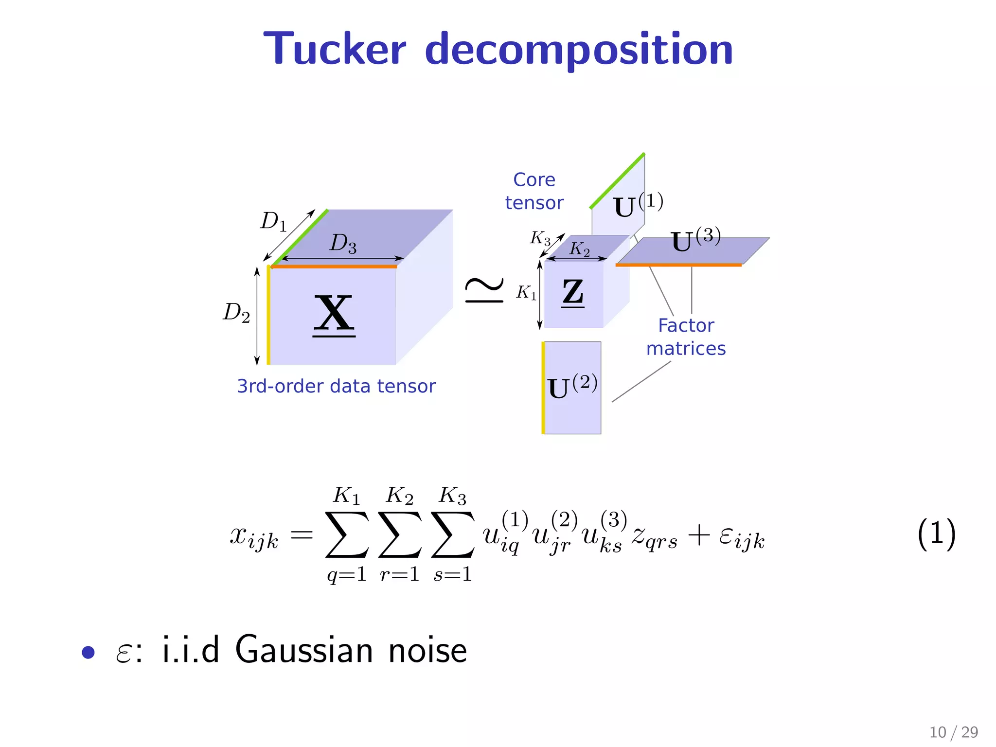
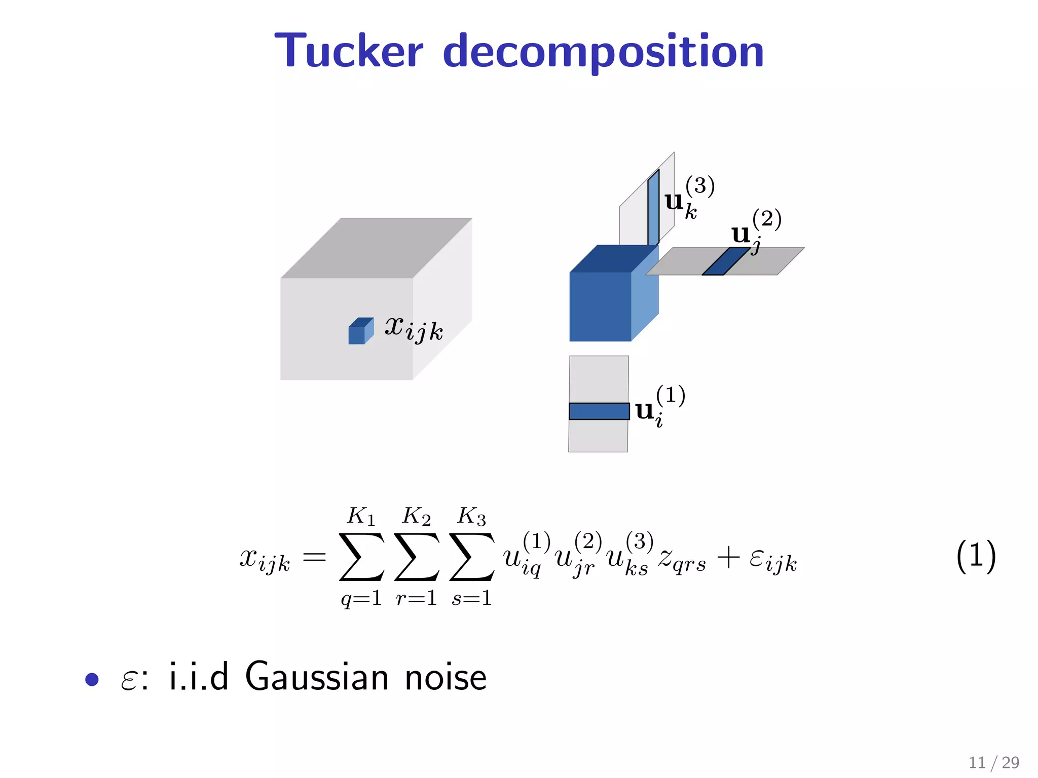
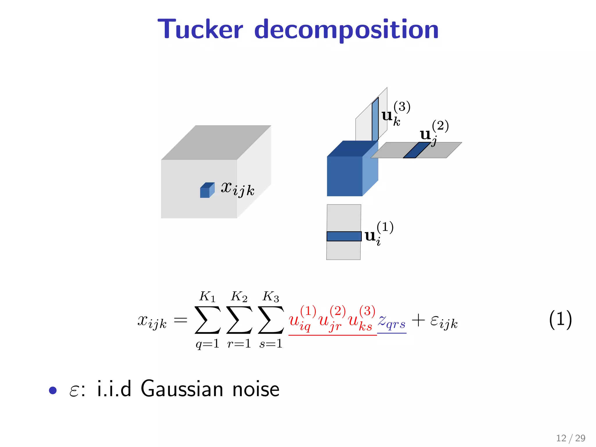
Tucker decomposition [Tucker 1966]: a tensor factorization
method assuming
1 observation noise is Gaussian
.
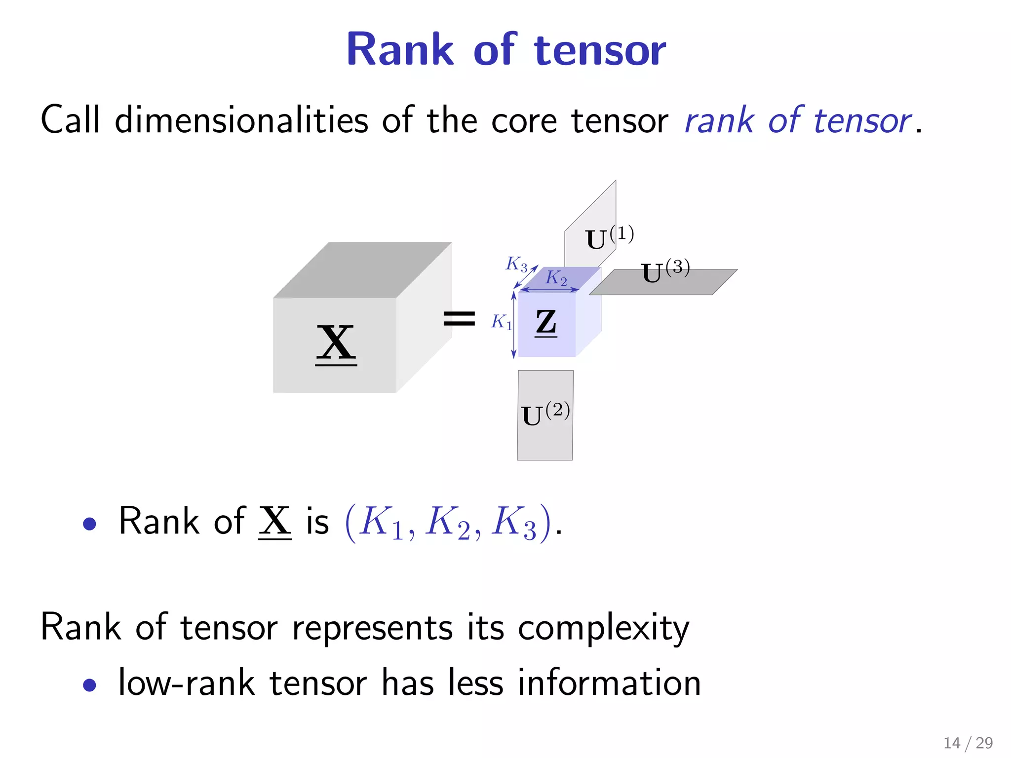
2 underlying tensor is low-dimensional
.
These assumptions are general ... but are not always
true.
6 / 29](https://image.slidesharecdn.com/short-120518210704-phpapp01/75/Generalization-of-Tensor-Factorization-and-Applications-6-2048.jpg)
![Contributions
Generalize Tucker decomposition and propose two new
models:
1 Exponential family tensor factorization (ETF)
.
[Joint work with Takenouchi, Shibata, Kamiya, Kunieda, Yamada, and
Ikeda]
• Generalize the noise distribution.
• Can handle a tensor containing mixed discrete and
continuous values.
2. Full-rank tensor completion (FTC)
[Joint work with Tomioka and Kashima]
• Kernelize Tucker decomposition
• Complete missing values without reducing the
dimensionality.
7 / 29](https://image.slidesharecdn.com/short-120518210704-phpapp01/75/Generalization-of-Tensor-Factorization-and-Applications-7-2048.jpg)
![Exponential family tensor factorization
.
Likelihood
.
D
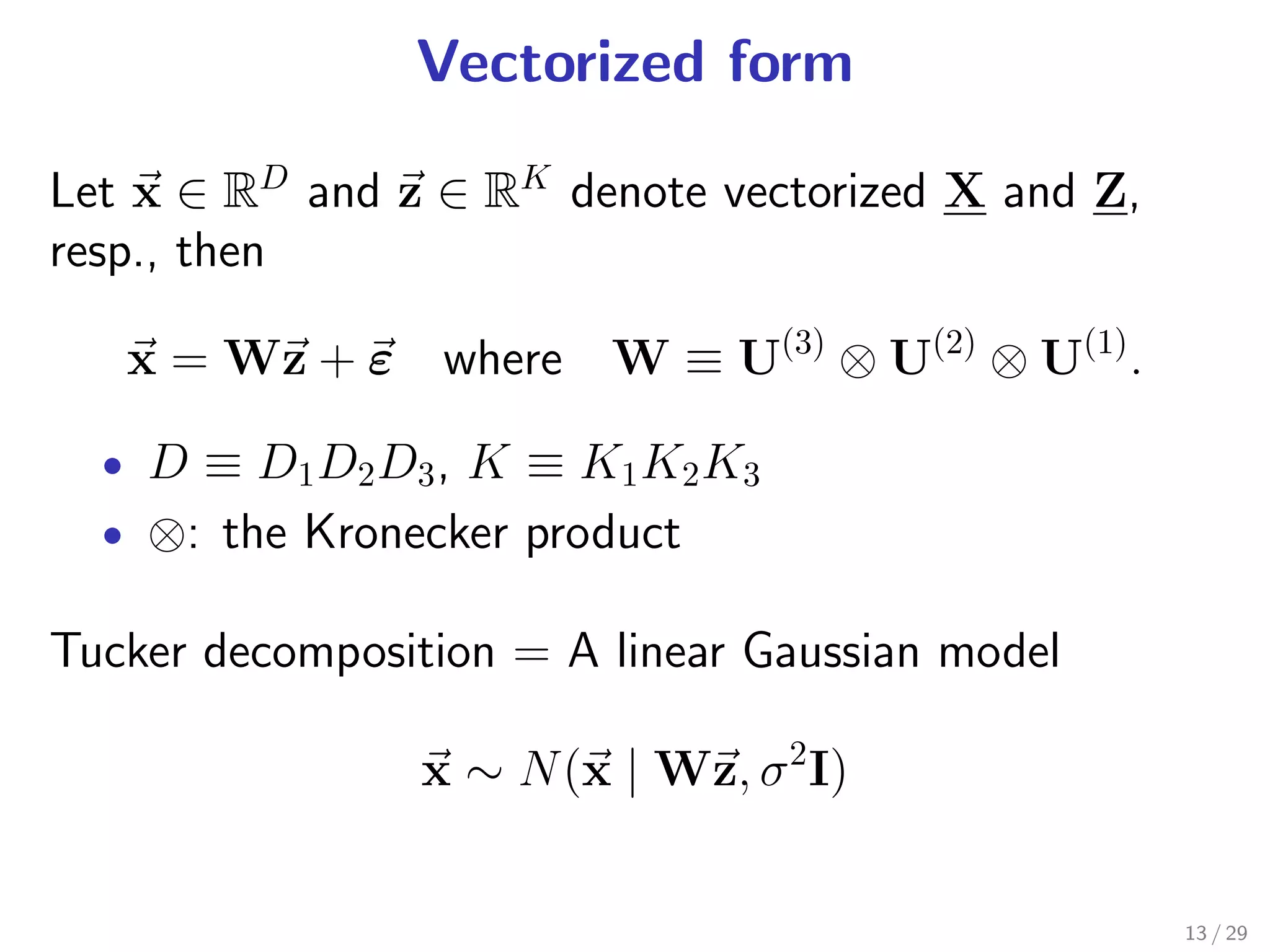
x∼ Expond (xd | θd ), θ ≡ Wz
d=1 exp. family Tucker decomp.
. where Expon(x | θ) ≡ exp [xθ − ψ(θ) + F (x)]
exponential family : a class of distributions
Gaussian Poisson Bernoulli
0.4
0.7
Density
Density
0.2
0.2
0.5
(θ = 0)
0.0
0.0
0.3
ψ(θ) θ2−4 −2
/2 0 2 4
exp[θ] 4
0 2 6 8
ln(10.0 0.5 1.0 1.5
−0.5
+ exp[θ])
x
18 / 29](https://image.slidesharecdn.com/short-120518210704-phpapp01/75/Generalization-of-Tensor-Factorization-and-Applications-18-2048.jpg)
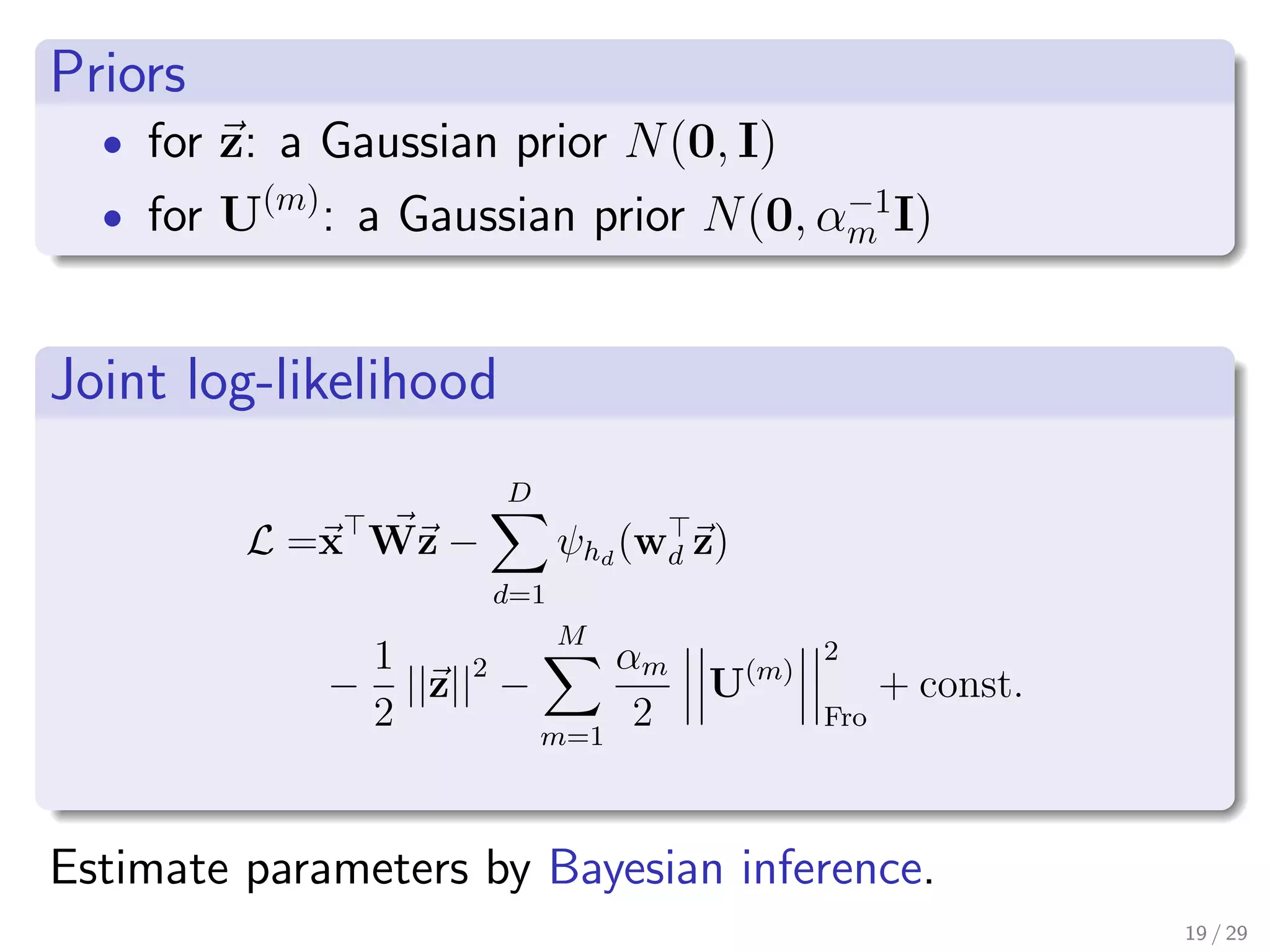
![Bayesian inference
Marginal-MAP estimator:
argmax exp[L(z, U(1) , . . . , U(M ) )]dz
U(1) ,...,U(M )
• The integral is not analytical.
Develop efficient yet accurate approximation with
Laplace approximation and Gaussian process.
• Computational cost is still higher than Tucker
dcomp.
• For a long and thin tensor (e.g. time series), online
algorithm is applicable (see thesis.)
20 / 29](https://image.slidesharecdn.com/short-120518210704-phpapp01/75/Generalization-of-Tensor-Factorization-and-Applications-20-2048.jpg)
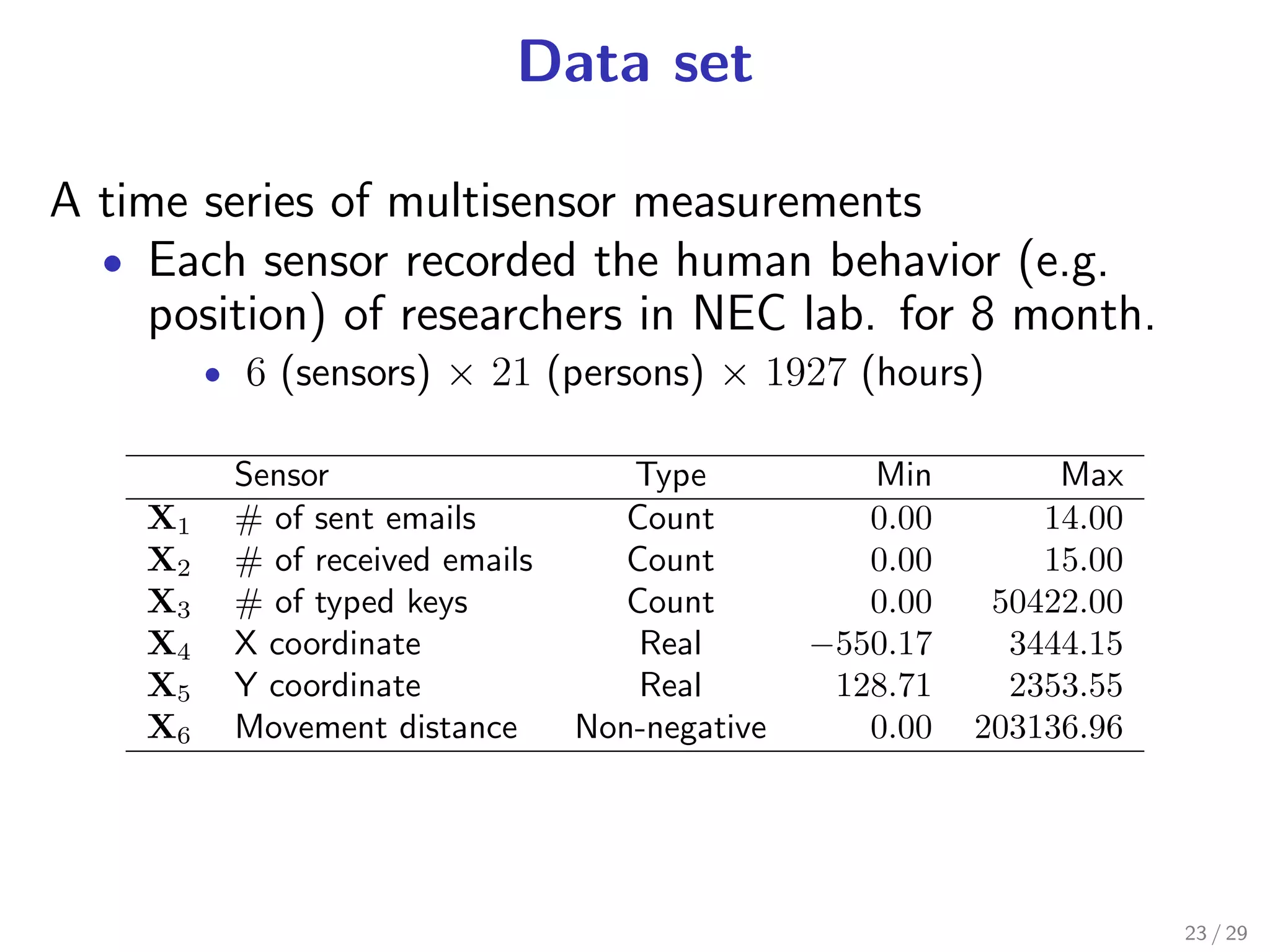
![Anomaly detection by ETF
Purpose Find irregular parts of tensor data
Method Apply distance-based outlier
DB (p, D) [Knorr+ VLDB’00] to the estimated
factor matrix U(m)
.
Definition of DB (p, D)
.
“An object O is a DB (p, D) outlier if at least fraction p
. the objects lies at a distance greater than D from O.”
of
22 / 29](https://image.slidesharecdn.com/short-120518210704-phpapp01/75/Generalization-of-Tensor-Factorization-and-Applications-22-2048.jpg)


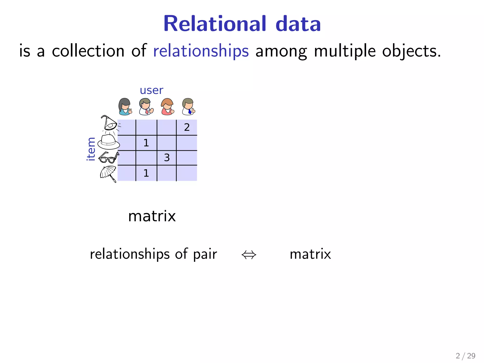
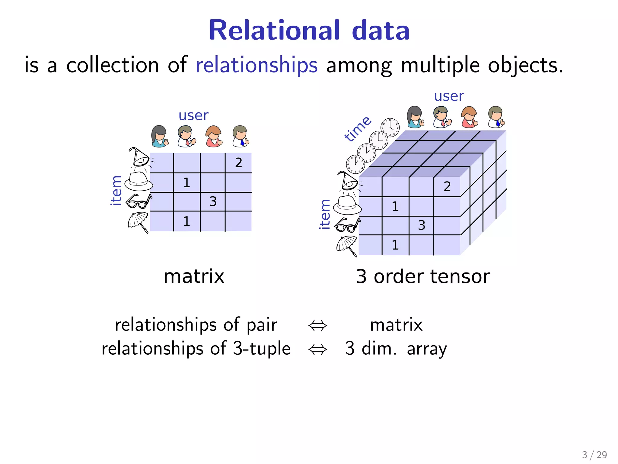
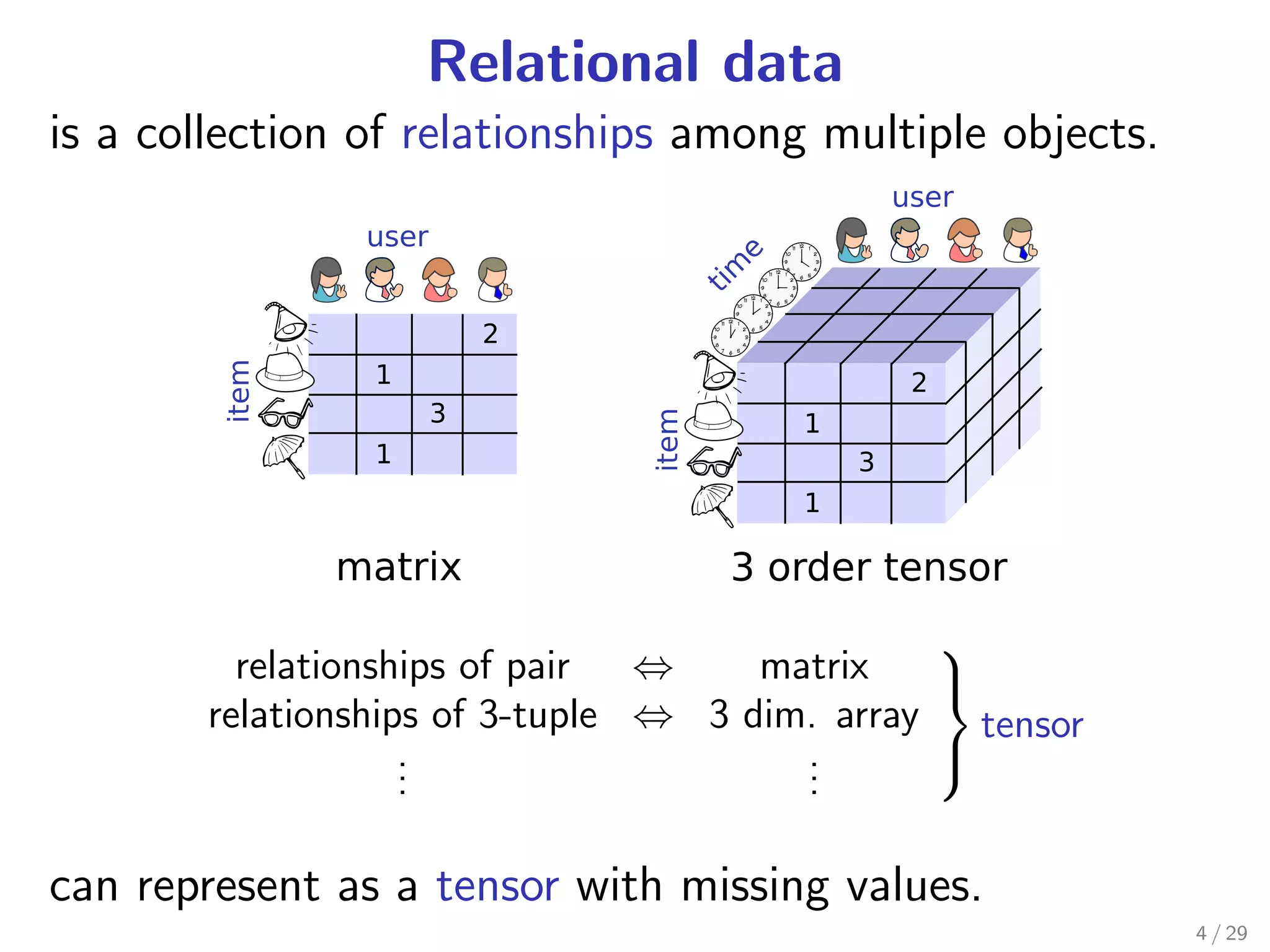
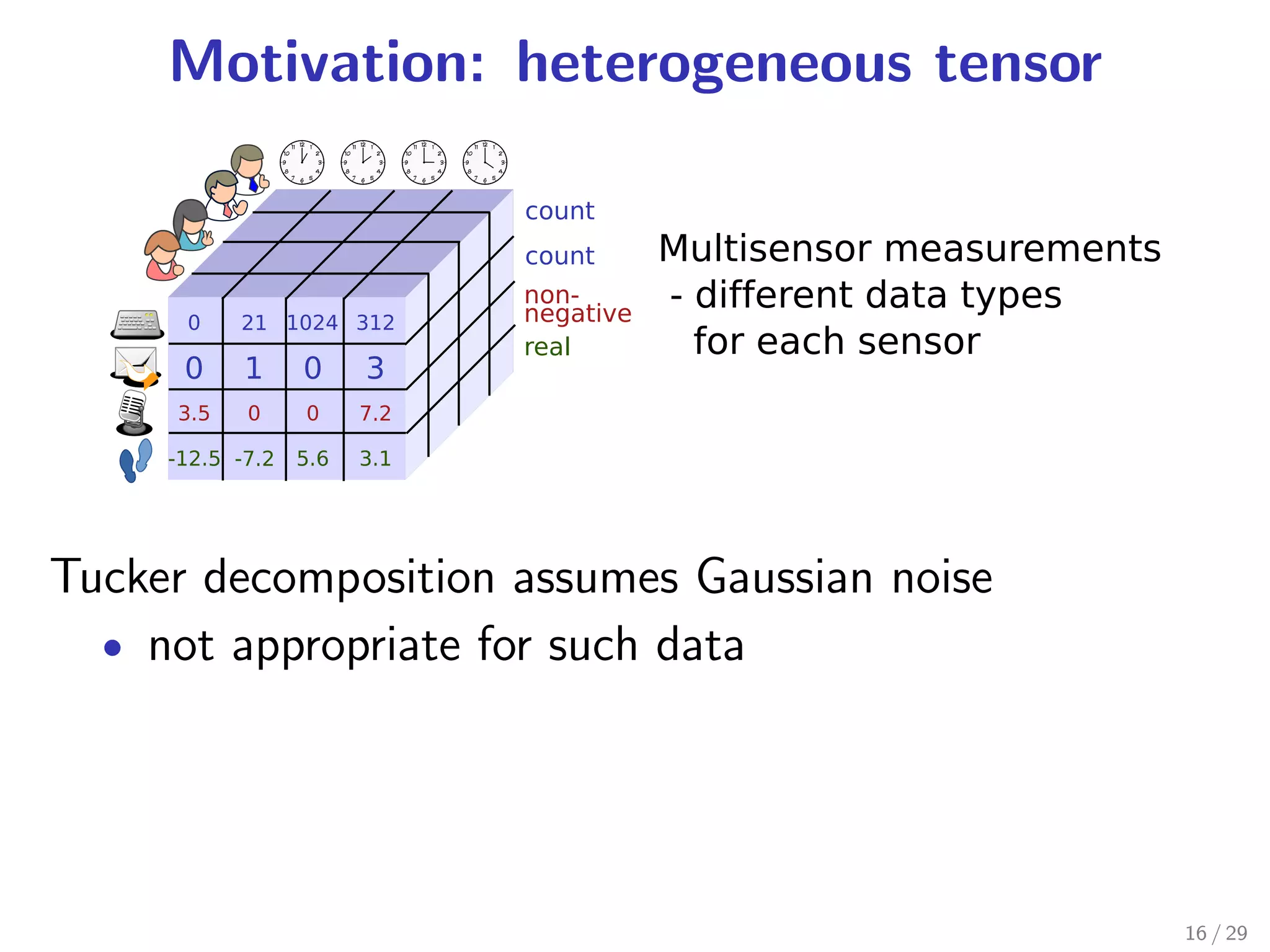
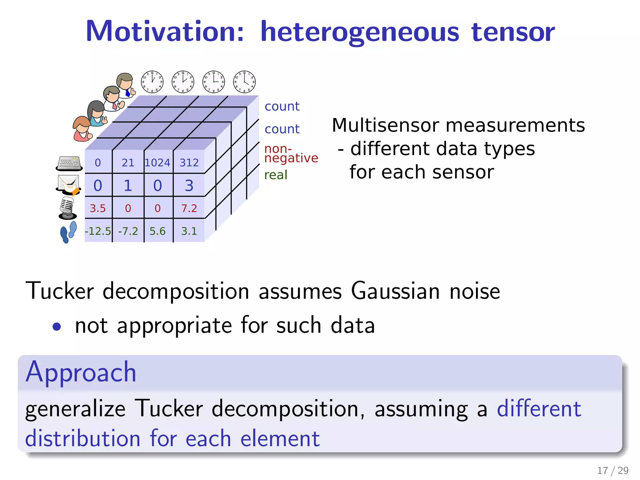
This document presents two tensor factorization methods: Exponential Family Tensor Factorization (ETF) and Full-Rank Tensor Completion (FTC). ETF generalizes Tucker decomposition by allowing for different noise distributions in the tensor and handles mixed discrete and continuous values. FTC completes missing tensor values without reducing dimensionality by kernelizing Tucker decomposition. The document outlines these methods and their motivations, discusses Tucker decomposition, and provides an example applying ETF to anomaly detection in time series sensor data.


![[DL輪読会]When Does Label Smoothing Help?](https://cdn.slidesharecdn.com/ss_thumbnails/yokota20191227dl-191227001522-thumbnail.jpg?width=640&height=640&fit=bounds)

![[DL輪読会]DisCo RL: Distribution-Conditioned Reinforcement Learning for General...](https://cdn.slidesharecdn.com/ss_thumbnails/210924dlseminarnakamoto-210924021720-thumbnail.jpg?width=640&height=640&fit=bounds)

![[DL輪読会]Convolutional Conditional Neural Processesと Neural Processes Familyの紹介](https://cdn.slidesharecdn.com/ss_thumbnails/20191220readingpaperconvcnp-191220034420-thumbnail.jpg?width=640&height=640&fit=bounds)


![[DL輪読会]DropBlock: A regularization method for convolutional networks](https://cdn.slidesharecdn.com/ss_thumbnails/dlyokota20190222-190222002832-thumbnail.jpg?width=640&height=640&fit=bounds)


![[DL輪読会]Learning to Generalize: Meta-Learning for Domain Generalization](https://cdn.slidesharecdn.com/ss_thumbnails/20180208-180209000942-thumbnail.jpg?width=640&height=640&fit=bounds)

![[DL輪読会]GLIDE: Guided Language to Image Diffusion for Generation and Editing](https://cdn.slidesharecdn.com/ss_thumbnails/glide2-220107030326-thumbnail.jpg?width=640&height=640&fit=bounds)


![[DL輪読会]Life-Long Disentangled Representation Learning with Cross-Domain Laten...](https://cdn.slidesharecdn.com/ss_thumbnails/20180914iwasawa-180919025635-thumbnail.jpg?width=640&height=640&fit=bounds)


![[DL輪読会]Conditional Neural Processes](https://cdn.slidesharecdn.com/ss_thumbnails/conditionalneuralprocesses-180727001730-thumbnail.jpg?width=640&height=640&fit=bounds)
![[DL輪読会]近年のエネルギーベースモデルの進展](https://cdn.slidesharecdn.com/ss_thumbnails/energybasedmodel-200124020855-thumbnail.jpg?width=640&height=640&fit=bounds)