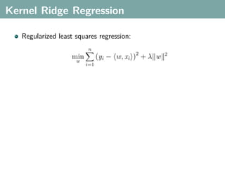
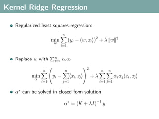
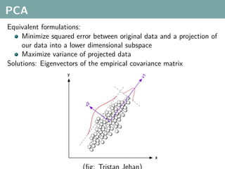
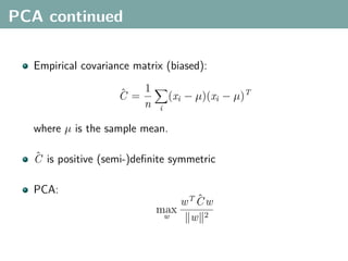
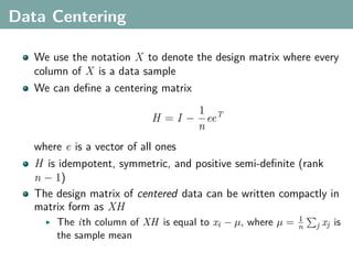
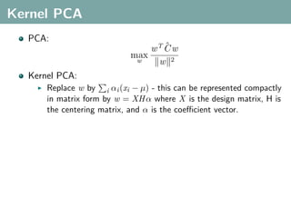
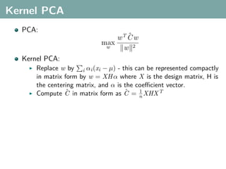
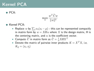
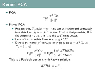
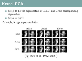
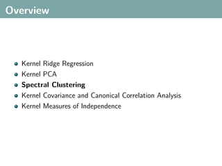
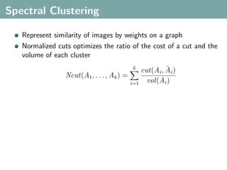
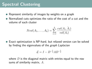
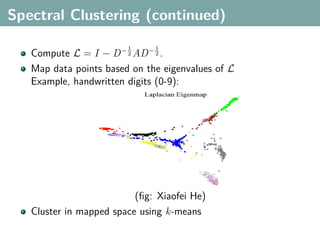
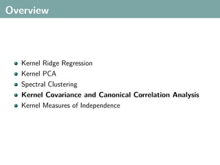
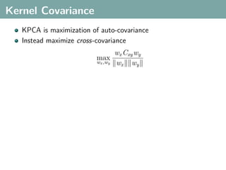
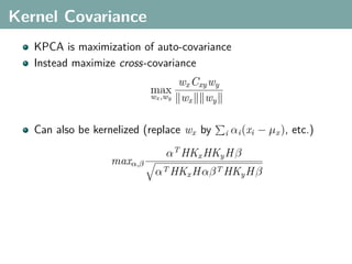
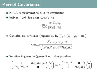
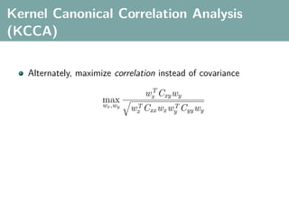
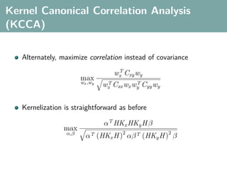
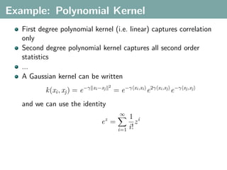
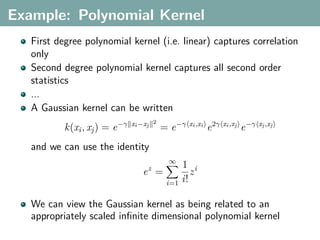
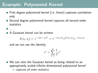
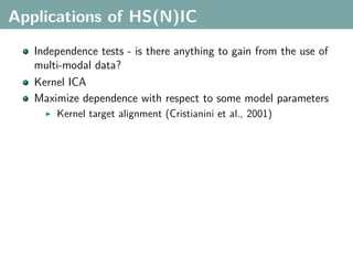
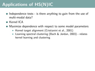
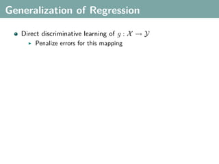
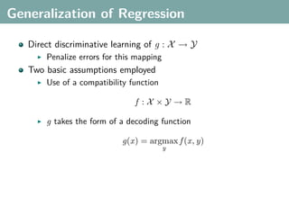
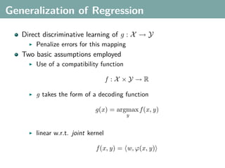
The document discusses several statistical and clustering techniques with kernels, including kernel ridge regression, kernel PCA, spectral clustering, kernel covariance/canonical correlation analysis, and kernel measures of independence. Kernel ridge regression performs regularized least squares regression in a reproducing kernel Hilbert space. Kernel PCA replaces the data vectors in regular PCA with representations in a reproducing kernel Hilbert space. Spectral clustering uses the eigenvectors of the graph Laplacian to map data points for clustering. Kernel covariance and canonical correlation analysis aim to maximize cross-covariance between different modalities in a reproducing kernel Hilbert space.

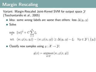
![Multimodal Data
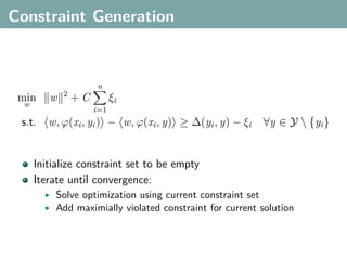
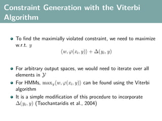
A latent aspect relates data that are present in multiple
modalities
e.g. images and text
XYZ[
_^]
z M
qqq MMM
qqq MMM
XYZ[
_^] _^]
XYZ[
q
x &
ϕx (x) ϕy (y) x:
y: “A view from Idyllwild, California,
with pine trees and snow capped Marion
Mountain under a blue sky.”](https://image.slidesharecdn.com/statisticsandclusteringwithkernelsslide-lampertblaschko-biologicalcybernetics-20092-110407220415-phpapp02/85/cvpr2009-tutorial-kernel-methods-in-computer-vision-part-II-Statistics-and-Clustering-with-Kernels-Structured-Output-Learning-20-320.jpg)
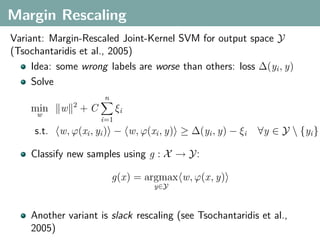
![Multimodal Data
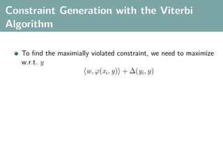
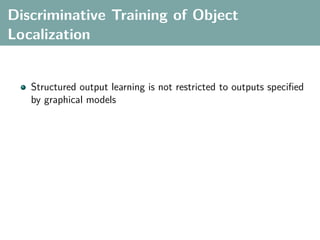
A latent aspect relates data that are present in multiple
modalities
e.g. images and text
XYZ[
_^]
z M
qqq MMM
qqq MMM
XYZ[
_^] _^]
XYZ[
q
x &
ϕx (x) ϕy (y) x:
y: “A view from Idyllwild, California,
with pine trees and snow capped Marion
Mountain under a blue sky.”
Learn kernelized projections that relate both spaces](https://image.slidesharecdn.com/statisticsandclusteringwithkernelsslide-lampertblaschko-biologicalcybernetics-20092-110407220415-phpapp02/85/cvpr2009-tutorial-kernel-methods-in-computer-vision-part-II-Statistics-and-Clustering-with-Kernels-Structured-Output-Learning-21-320.jpg)
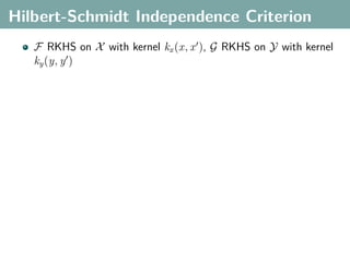
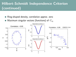
![Hilbert-Schmidt Independence Criterion
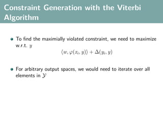
F RKHS on X with kernel kx (x, x ), G RKHS on Y with kernel
ky (y, y )
Covariance operator: Cxy : G → F such that
f , Cxy g F = Ex,y [f (x)g(y)] − Ex [f (x)]Ey [g(y)]](https://image.slidesharecdn.com/statisticsandclusteringwithkernelsslide-lampertblaschko-biologicalcybernetics-20092-110407220415-phpapp02/85/cvpr2009-tutorial-kernel-methods-in-computer-vision-part-II-Statistics-and-Clustering-with-Kernels-Structured-Output-Learning-43-320.jpg)
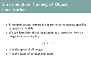
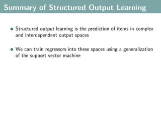
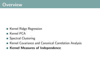
![Hilbert-Schmidt Independence Criterion
F RKHS on X with kernel kx (x, x ), G RKHS on Y with kernel
ky (y, y )
Covariance operator: Cxy : G → F such that
f , Cxy g F = Ex,y [f (x)g(y)] − Ex [f (x)]Ey [g(y)]
HSIC is the Hilbert-Schmidt norm of Cxy (Fukumizu et al. 2008):
2
HSIC := Cxy HS](https://image.slidesharecdn.com/statisticsandclusteringwithkernelsslide-lampertblaschko-biologicalcybernetics-20092-110407220415-phpapp02/85/cvpr2009-tutorial-kernel-methods-in-computer-vision-part-II-Statistics-and-Clustering-with-Kernels-Structured-Output-Learning-44-320.jpg)
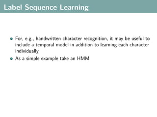
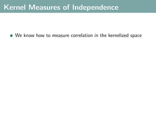
![Hilbert-Schmidt Independence Criterion
F RKHS on X with kernel kx (x, x ), G RKHS on Y with kernel
ky (y, y )
Covariance operator: Cxy : G → F such that
f , Cxy g F = Ex,y [f (x)g(y)] − Ex [f (x)]Ey [g(y)]
HSIC is the Hilbert-Schmidt norm of Cxy (Fukumizu et al. 2008):
2
HSIC := Cxy HS
(Biased) empirical HSIC:
1
HSIC := Tr(Kx HKy H )
n2](https://image.slidesharecdn.com/statisticsandclusteringwithkernelsslide-lampertblaschko-biologicalcybernetics-20092-110407220415-phpapp02/85/cvpr2009-tutorial-kernel-methods-in-computer-vision-part-II-Statistics-and-Clustering-with-Kernels-Structured-Output-Learning-45-320.jpg)
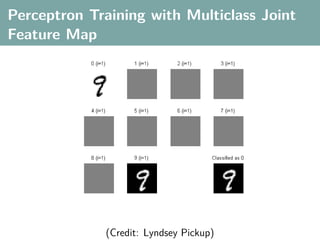
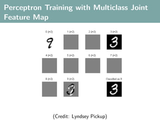
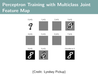
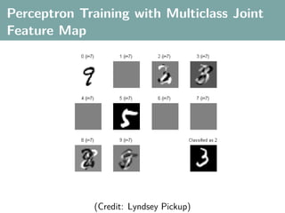
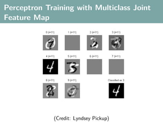
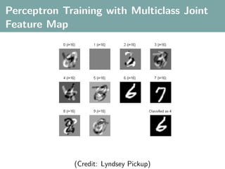
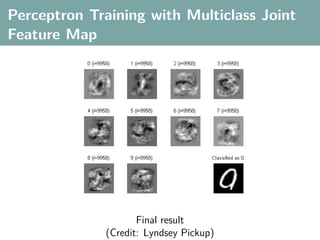
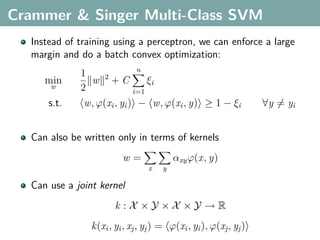
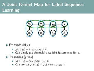
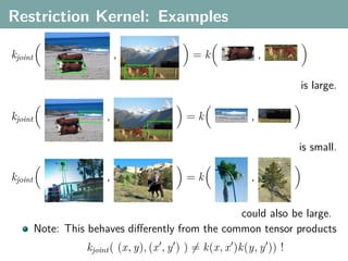
![Multi-Class Joint Feature Map
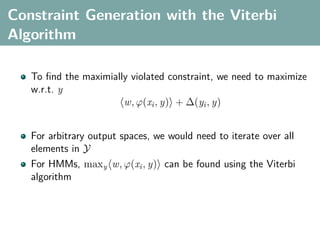
Simple joint kernel map:
define ϕy (yi ) to be the vector with 1 in place of the current
class, and 0 elsewhere
ϕy (yi ) = [0, . . . , 1 , . . . , 0]T
kth position
if yi represents a sample that is a member of class k](https://image.slidesharecdn.com/statisticsandclusteringwithkernelsslide-lampertblaschko-biologicalcybernetics-20092-110407220415-phpapp02/85/cvpr2009-tutorial-kernel-methods-in-computer-vision-part-II-Statistics-and-Clustering-with-Kernels-Structured-Output-Learning-69-320.jpg)
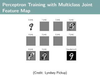
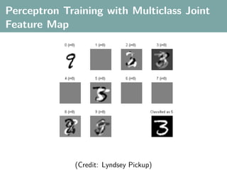
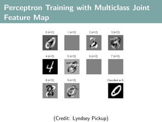
![Multi-Class Joint Feature Map
Simple joint kernel map:
define ϕy (yi ) to be the vector with 1 in place of the current
class, and 0 elsewhere
ϕy (yi ) = [0, . . . , 1 , . . . , 0]T
kth position
if yi represents a sample that is a member of class k
ϕx (xi ) can result from any kernel over X :
kx (xi , xj ) = ϕx (xi ), ϕx (xj )](https://image.slidesharecdn.com/statisticsandclusteringwithkernelsslide-lampertblaschko-biologicalcybernetics-20092-110407220415-phpapp02/85/cvpr2009-tutorial-kernel-methods-in-computer-vision-part-II-Statistics-and-Clustering-with-Kernels-Structured-Output-Learning-70-320.jpg)
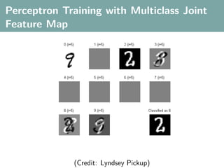
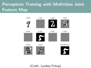
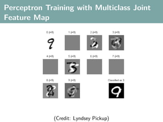
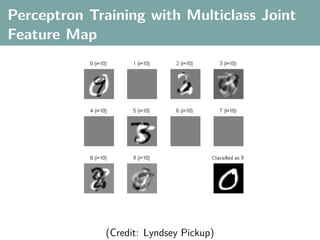
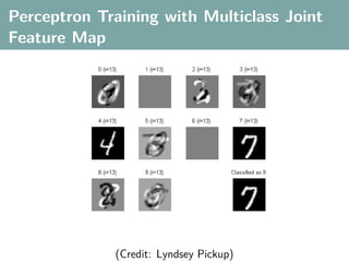
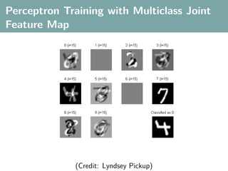
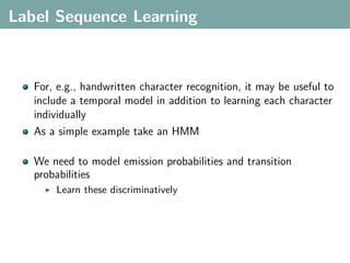
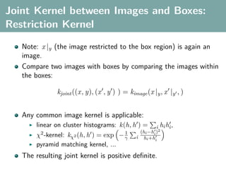
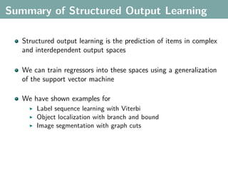
![Multi-Class Joint Feature Map
Simple joint kernel map:
define ϕy (yi ) to be the vector with 1 in place of the current
class, and 0 elsewhere
ϕy (yi ) = [0, . . . , 1 , . . . , 0]T
kth position
if yi represents a sample that is a member of class k
ϕx (xi ) can result from any kernel over X :
kx (xi , xj ) = ϕx (xi ), ϕx (xj )
Set ϕ(xi , yi ) = ϕy (yi ) ⊗ ϕx (xi ), where ⊗ represents the
Kronecker product](https://image.slidesharecdn.com/statisticsandclusteringwithkernelsslide-lampertblaschko-biologicalcybernetics-20092-110407220415-phpapp02/85/cvpr2009-tutorial-kernel-methods-in-computer-vision-part-II-Statistics-and-Clustering-with-Kernels-Structured-Output-Learning-71-320.jpg)