11.generalized and subset integrated autoregressive moving average bilinear time series models

Journal of Economics and Sustainable Development www.iiste.org
ISSN 2222-1700 (Paper) ISSN 2222-2855 (Online)
Vol.3, No.4, 2012

Generalized and Subset Integrated Autoregressive Moving

Average Bilinear Time Series Models

Ojo J. F.
Department of Statistics, University of Ibadan, Ibadan, Nigeria
Tel: +2348033810739 E-mail: jfunminiyiojo@yahoo.co.uk
Abstract

Generalized integrated autoregressive moving average bilinear model which is capable of achieving
stationary for all non linear series is proposed and compared with subset generalized integrated
autoregressive moving average bilinear model using the residual variance to see which perform better.
The parameters of the proposed models are estimated using Newton-Raphson iterative method and
Marquardt algorithm and the statistical properties of the derived estimates were investigated. An
algorithm was proposed to eliminate redundant parameters from the full order generalized integrated
autoregressive moving average bilinear models. To determine the order of the models, Akaike
Information Criterion (AIC) and Bayesian Information Criterion (BIC) were adopted. Generalized
integrated autoregressive moving average bilinear models are fitted to Wolfer sunspot numbers and
stationary conditions are satisfied. Generalized integrated autoregressive moving average bilinear
model performed better than subset generalized integrated autoregressive bilinear model.
Keywords: Stationary, Newton-Raphson, Residual Variance, Marquardt Algorithm and
Parameters.

1. Introduction
The bilinear time series models have attracted considerable attention during the last years. An overview
of bilinear models and their application can be found in (Subba Rao 1981), (Pham & Tran 1981), (Gabr
& Subba Rao 1981), (Rao et al. 1983), (Liu 1992), (Gonclaves et al. 2000), (Shangodoyin & Ojo
2003), (Wang & Wei 2004), (Boonaick et al.2005), (Bibi 2006), (Doukhan et al. 2006), (Drost et al.
2007), (Usoro & Omekara 2008) and (Ojo 2009). The bilinear modes studied by the above researchers
could not achieve stationary for all nonlinear series. One-dimensional bilinear time series model that
could achieve stationary for all non linear series was developed, for details see (Shangodoyin et al.
2010) and (Ojo 2010). In this paper we proposed generalized integrated autoregressive moving average
and subset integrated autoregressive moving average bilinear time series models that could achieve
stationary for all non linear real series.

2. Proposed Generalized Integrated Autoregressive Moving average Bilinear Time Series Models
We define generalized bilinear (GBL) and generalized subset bilinear (GSBL) time series models as

follows:

Model 1(M1)

r s
ψ ( B) X t = φ ( B)∇ d X t + θ ( B)et + ∑∑ bkl X t −k et −l , denoted as GBL (p, d, q, r, s)
k =1 l =1

where φ ( B) = 1 − φ1 B − φ 2 B 2 ....... − φ p B p , θ ( B) = 1 − θ1 B − θ 2 B 2 ......... − θ q B q and
X t = ψ 1 X t −1 + ...... + ψ p+d X t − p−d + et − θ1et −1 − ...... − θ q et −q + b11 X t −1et −1 + ....... + brs X t −r et −s

23

Vol.3, No.4, 2012

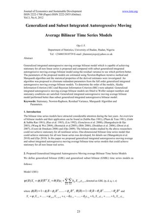
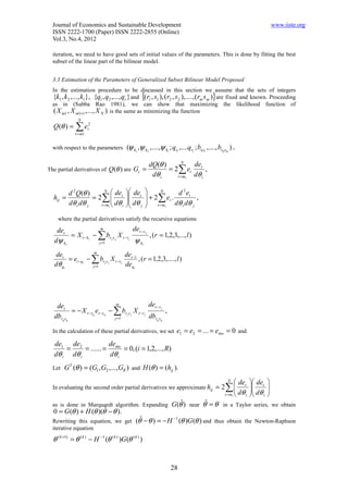
φ1 ,...,φ p are the parameters of the autoregressive component; θ1 ,...θ q are the parameters of the
associated error process; b11 ,........., brs are the parameters of the non-linear component and θ (B ) is
the moving average operator; p is the order of the autoregressive component; q is the order of the
moving average process; r, s is the order of the nonlinear component and ψ ( B) = ∇ φ ( B) is the
d

generalized autoregressive operator; ∇ is the differencing operator and d is the degree of consecutive
d

differencing required to achieve stationary. et are independently and identically distributed as N (0, σ e )
2

and the models are assume to be invertible.
Model 2 (M2)

l m n
X t = ∑ψ pi +d X t − pi −d − ∑θ q j et −q j + ∑ brk sk X t −rk et −sk + et ,
i =1 j =1 k =1

The above equation is denoted as GSBL (p, d, q, r, s) and pi is the order of subset autoregressive

integrated component, qj is the order of subset moving average component and rk sk is the order of

subset nonlinear component. In the models above, et are independently and identically distributed as N

(0, σ e ) and the models are assume to be invertible.
2

3. Stationary and Convergence of GBL (p, d, q, r, s)
For general S, it is not easy to provide an infinite series representation for each X t . For this general
case, we exhibit the process { X t , t ∈ Z ) as an almost sure limit of a sequence
{{S n ,t , t ∈ Z }, n ≥ 1} of stationary processes.
Theorem
{ }
Let et , t ∈ Z be a sequence of independent identically distributed random variables defined on a
( )
probability space Ω, IR, P such that E et = 0 and Eet = σ < ∞ . Ψ , Θ, B1, B2,….,Bq be q+1
2 2

matrices each of order p x p.
Γ1 = (Ψ ⊗ Ψ + σ ((Θ ⊗ Θ + B ⊗ B) − 2Θ ⊗ B)
2
)
Γi = σ [ Bi ⊗ (Ψ j −1 B1 + Ψ j −2 B2 + ...... + ΨB j −1 )
2

+ (Ψ i −1 B1 + Ψ i −2 B2 + ... + ΨBi −1 ) ⊗ B j
+ Bi ⊗ (Θ j −1 B1 + Θ j −2 B2 + ....... + ΘB j −1 )
+ (Θ i −1 B1 + Θ i −2 B2 + ..... + ΘBi −1 ) ⊗ B j
+ ( B j ⊗ B j )], j = 2, 3,……s.
Suppose all the eigenvalues of the matrix

 Γ1 Γ2 ....... Γq−1 Γq 
 
I 2 0 ....... 0 0
L2 = p
p 2 q× p q 0 I p2 ...... 0 0
 
 0 0 I p2 ..... 0 
 
have moduli less than unity, i.e, ρ ( L ) = λ < 1. Let C be a given column vector. Then there exists
{
a vector valued strictly stationary process X t , t ∈ Z px1
s
}
conforming to the bilinear model
X t = ΨX t −1 − Θet −1 + ∑ B l X t −1et −1 + Cet for every t in Z.
l =1

24

Vol.3, No.4, 2012

Proof
Let the process {S n ,t , n, t ∈ Z } be defined as follows.
S n ,t = 0, if n < 0,
= Cet, if n = 0,
= Cet + (Ψ − Θet −1 + B1et −1 ) S n −t ,t −1 + B2 S n − 2,t − 2 et −2 + ... + Bq S n − q ,t −q et − q , if n>0
for every t in Z.
lim n→∞ S n ,t exists almost surely for every t in Z. If Xt is the almost sure limit of {S n ,t , n ≥ 1} for

every t in Z, then it is obvious that the process { X t , t ∈ Z } conforms to the bilinear model

X t = ψ 1 X t −1 + ...... + ψ p+d X t − p−d + et − θ1et −1 − ...... − θ q et −q + b11 X t −1et −1 + ....... + brs X t −r et −s

Also, for every fixed n in Z, {S
t ∈ Z } is a strictly stationary process.
n ,t ,
Let s n ,t = S n ,t − S n −1,t , t ∈ Z . E ( s n ,t ) i ≤ Kλ for every n ≥ 0 and i = 1, 2, ….,p, where K is a
n/2

positive constant. Since λ < 1, this then implies that {S n ,t , n ≥ 1} converges almost surely for every t
in Z.

3.1Algorithm for Fitting One-dimensional Autoregressive Integrated Moving Average Bilinear Time
Series Models

For the sake of simplicity, we will break the algorithm down into the following steps.

Step 1
Fit various order of autoregressive integrated moving average model of the form
X t = ψ 1 X t −1 + ...... + ψ p + d X t − p −d − θ1et −1 − ... − θ q et −q + et

Step 2
Choose the model for which Akaike Information Criterion (AIC) is minimum among various order
fitted in step 1.

Step 3
Fit possible subsets of chosen model in step 2 using 2 q − 1 subsets approach (Hagan & Oyetunji 1980).

Step 4
Choose the model for which AIC is minimum among the fitted models in step 3 to have the best subset
model and the parameters of this model form the initial values.

Step 5
Fit various order of generalized autoregressive integrated moving average bilinear model of the
form X t = ψ 1 X t −1 + ...... + ψ p +d X t − p−d − θ1et −1 − .... − θ q et −q + b11 X t −1et −1 + ........ + brs X t −r et − s + et

Step 6
Fit possible subsets of chosen model in step 5 using 2 q − 1 subsets approach (Shangodoyin & Ojo
2003)

25

Vol.3, No.4, 2012

Step 7 The model with the minimum AIC is the generalized subset autoregressive integrated moving
average bilinear model.
3.2 Estimation of the Parameters of Generalized Bilinear Models Proposed

The joint density function of (em , em +1 ,...., e n ) where m = max (r, s) is given by
1 1 n 2
(2πσ e2 )( n − m +1) / 2
exp( ∑ et )
− 2σ e2 m
Since the Jacobian of the transformation from (e m , e m +1 ,...., e n ) to ( X m , X m +1 ,...., X n ) is unity,
the likelihood function of ( X m , X m +1 ,...., X n ) is the same as the joint density function of
(em , em+1 ,...., e n ) . Maximising the likelihood function is the same as minimizing the function
Q (G ) ,
n
where Q (G ) = ∑ et2, (1)
i=m

with respect to the parameter G = (ψ 1 ,....,ψ p ;θ 1 ,θ 2 ,....,θ q ; B11 ,...., B rs )
'

Then the partial derivatives of Q(G) are given by
n
dQ(G ) de
= 2∑ et t (i = 1, 2,…..,R) (2)
dGi t =m dGi

d 2Q(G ) n
det det n
d 2et
= 2(∑ et + ∑ et )
dGi dG j t =m dGi dG j t = m dGi dG j

where these partial derivatives of e(t) satisfy the recursive equations

det s det − j
+ ∑ Wt (t ) = 1, if i = 0
dψ i j =1 dψ i
Xt-i , if i = 1, 2, …, p (3)
det s det − j
+ ∑Wt (t ) = et − i , if i = 1, 2,….., q (4)
dθ i j =1 dθ i

det s det − j
+ ∑W j (t ) = − X t − k et − m (k=1,2,…,r ; mi =1,2,…,s) (5)
dBkmi j =1 dBkmi

d 2 et s d 2 et − j
+ ∑ W j (t ) = 0 (i, i' = 0, 1, 2, …, p) (6)
dψ i dψ i' j =1 dψ i dψ i'

d 2et s d 2et − j
+ ∑W j (t ) =0 (i, i' = 0, 1, 2, …, q) (7)
dθ i dθ i' j =1 dθ i dθ i'

26

Vol.3, No.4, 2012

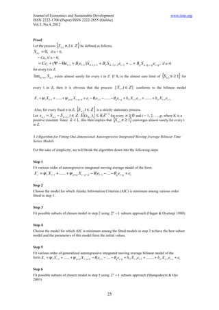
d 2 et s d 2 et − j d 2 et − mi
+ ∑ W j (t ) + X t −k =0
dψ i dBkmi j =1 dBkmi dφ i dψ i
(i=0,1,2,…,p ; ki =1,2,…,r; mi=1,2,…,s) (8)

d 2et s d 2et − j d 2et − mi
+ ∑W j (t ) + X t −k =0
dθ i dBkmi j =1 dBkmi dθ i dθ i

(i=1,2,…,q ; ki =1,2,…,r; mi=1,2,…,s) (9)

d 2et s d 2et − j
+ ∑ W j (t ) =0
dψ i dθi j =1 dψ i dθi
(10)

d 2 et s d 2 et − j d 2 e t − mi de
'
+ ∑ W j (t ) '
+ X t' − k = − X t −k t −m
'
dB kmi dB kmi j =1 dB kmi dB kmi dB kmi dB kmi

(k, k' =1,2,…,r ; mi mi' = 1,2,…,s)
(11)

s
W j (t ) = ∑ Bij X t − j We assume et = 0 (t = 1, 2, …, m-1) and also
j =1

det d 2et
= 0, = 0, (i, j = 1, 2, …, R; t = 1, 2, …, m-1)
dGi dGi dG j

From et=0 (t= 1, 2, …, m-1),

det d 2et det s det − j
= 0, = 0 , and + ∑W j (t ) = − X t − k et − m (k=1,2,…,r ; mi =1,2,…,s),
dGi dGi dG j dBkmi j =1 dBkmi
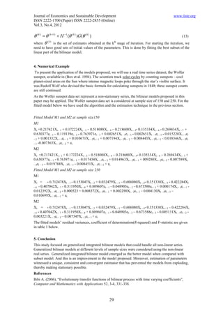
it

follows that the second order derivatives with respect to ψ i (i = 0, 1, 2, …, p) and θi (i = 0, 1, 2, …,
q) are zero. For a given set of values {φi}, { θi } and {Bij } one can evaluate the first and second order
derivatives using the recursive equations 3, 4, 5 and 11. Now let

dQ (G ) dQ (G ) dQ(G )
V ' (G ) = , ,........,
dG 1 dG 2 dG k

and let H (G ) = [ d Q (G ) / dG i dG j ] be a matrix of second partial derivatives as in (Krzanowski
2

1998). Expanding V(G), near G = G in a Taylor series, we obtain
ˆ
V (G ) G =G = 0 = V (G ) + H (G )(G − G )
ˆ ˆ ˆ
(12)
−1
Rewriting this equation we get G − G = − H (G )V (G ), and thus obtain an iterative equation given
ˆ
( k +1) −1
by G = G − H (G )V (G ( k ) ) where G (k ) is the set of estimates obtained at the kth stage
(k ) (k )

of iteration. The estimates obtained by the above iterative equations usually converge. For starting the

27

Vol.3, No.4, 2012

iteration, we need to have good sets of initial values of the parameters. This is done by fitting the best
subset of the linear part of the bilinear model.

3.3 Estimation of the Parameters of Generalized Subset Bilinear Model Proposed
In the estimation procedure to be discussed in this section we assume that the sets of integers
{ }
{k1 , k2 ,..., kl }, {q1 , q2 ,..., qr } and (r1 , s1 ), (r2 , s 2 ),...., (rm s m ) are fixed and known. Proceeding
as in (Subba Rao 1981), we can show that maximizing the likelihood function of
( X m1 , X m1+1 ,..., X N ) is the same as minimizing the function
N
Q (θ ) = ∑e
t = m1
2
t

with respect to the parameters (ψ k1 ,ψ k2 ,....,ψ kl ; qr1 ,....qrz ; br1s1 ,...., brmsm ) .

dQ(θ ) N
de
The partial derivatives of Q (θ ) are Gi = = 2 ∑ et t ,
dθ i t = m1 dθ i

d 2 Q(θ ) N
 de  det  N 2
hij = = 2∑ t   + 2 ∑ et . d et ,
dθ i dθ j   dθ  t = m dθ dθ
t = m1  dθ i  j  1 i j

where the partial derivatives satisfy the recursive equations

det m det − s j
= X t − k r − ∑ br j s j X t − r j , (r = 1,2,3,..., l )
dψ k r j =1 ψ kr
m
det de
= et −qr − ∑ brj s j X t −rj t −1 , ( r = 1,2,3,...., l )
d θ qr j =1 deqr

det m det − s j
= − X t −rq et − sq − ∑ br j s j X t − r j ,
dbrq sq j =1 dbrq sq

In the calculation of these partial derivatives, we set e1 = e2 = ... = emo = 0 and
de1 de2 de
= = ...... = mo = 0, (i = 1,2,..., R)
dθ i dθ i dθ i
Let GT (θ ) = (G1 , G2 ,..., GR ) and H (θ ) = (hij ).
N
 de  det 
In evaluating the second order partial derivatives we approximate hij = 2∑  t  
 dθ 

t = m1  dθ i  i 
as is done in Marquardt algorithm. Expanding G(θ ) near θ = θ in a Taylor series, we obtain
ˆ ˆ
0 = G (θ ) + H (θ )(θ − θ ).
ˆ
Rewriting this equation, we get (θ − θ ) = − H −1 (θ )G (θ ) and thus obtain the Newton-Raphson
ˆ
iterative equation
θ ( k +1) = θ ( k ) − H −1 (θ ( k ) )G (θ ( k ) )

28

Vol.3, No.4, 2012

θ ( k ) = θ ( k +1) + H −1 (θ ( k ) )G (θ ( k ) ) (13)
where θ
(k )
is the set of estimates obtained at the kth stage of iteration. For starting the iteration, we
need to have good sets of initial values of the parameters. This is done by fitting the best subset of the
linear part of the bilinear model.

4. Numerical Example
To present the application of the models proposed, we will use a real time series dataset, the Wolfer
sunspot, available in (Box et al. 1994). The scientists track solar cycles by counting sunspots – cool
planet-sized areas on the Sun where intense magnetic loops poke through the star’s visible surface. It
was Rudolf Wolf who devised the basic formula for calculating sunspots in 1848; these sunspot counts
are still continued.
As the Wolfer sunspot data set represent a non-stationary series, the bilinear models proposed in this
paper may be applied. The Wolfer sunspot data set is considered at sample size of 150 and 250. For the
fitted model below we have used the algorithm and the estimation technique in the previous section.

Fitted Model M1 and M2 at sample size150
M1
Xt =0.217421Xt – 1 + 0.172224Xt – 3 – 0.518088Xt – 4 – 0.218600Xt – 5- 0.135334Xt – 6 - 0.269434Xt – 7 +
0.630377et - 1 – 0.119139et – 2 - 0.763971et – 3 + 0.002651Xt – 1et – 1 - 0.002651Xt – 1et – 1 - 0.015220Xt – 1et
– 2 + 0.001332Xt – 1et – 3 + 0.010671Xt – 2et – 1 + 0.007194Xt – 2et – 2 – 0.008443Xt – 2et – 3 – 0.018346Xt – 3et
– 1 -0.007363Xt – 3et – 2 + et

M2
Xt =0.217421Xt – 1 + 0.172224Xt – 3 – 0.518088Xt – 4 – 0.218600Xt – 5- 0.135334Xt – 6 – 0.269434Xt – 7 +
0.630377et – 1 - 0.763971et – 3 – 0.017434Xt – 1et – 2 + 0.014963Xt – 2et – 1 + 009280Xt – 2et – 2 - 0.007589Xt
– 2et – 3 – 0.019788Xt – 3et – 1 - 0.008451Xt – 3et – 2 + et

Fitted Model M1 and M2 at sample size 250
M1
Xt = - 0.712478Xt – 1 - 0.153047Xt – 2 + 0.032479Xt – 3 – 0.606080Xt – 4- 0.351330Xt – 5 - 0.422284Xt
– 6 - 0.407042Xt - 7 - 0.311950Xt – 8 + 0.809607et – 1 - 0.048903et – 2 - 0.673588et – 3 + 0.000174Xt – 1et – 1 -
0.012392Xt – 1et – 2 - 0.000523 + 0.008372Xt – 2et – 1 + 0.002290Xt – 2et - 2 – 0.004130Xt – 2et – 3 –
0.010699Xt – 3et – 1 + et
M2
Xt = - 0.712478Xt – 1 - 0.153047Xt – 2 + 0.032479Xt – 3 – 0.606080Xt – 4- 0.351330Xt – 5 – 0.422284Xt
–6 - 0.407042Xt – 7 - 0.311950Xt – 8 + 0.809607et – 1 - 0.048903et – 2 – 0.673588et – 3 - 0.005131Xt – 1et – 2 -
0.003221Xt – 2et – 3 – 0.007347Xt – 3et – 1 + et
The fitted models’ residual variances, coefficient of determination(R-squared) and F-statistic are given
in table 1 below.

5. Conclusion
This study focused on generalized integrated bilinear models that could handle all non-linear series.
Generalized bilinear models at different levels of sample sizes were considered using the non-linear
real series. Generalized integrated bilinear model emerged as the better model when compared with
subset model. And this is an improvement in the model proposed. Moreover, estimation of parameters
witnessed a unique, consistent and convergent estimator that has prevented the models from exploding,
thereby making stationary possible.
References
Bibi A. (2006), “Evolutionary transfer functions of bilinear process with time varying coefficients”,
Computer and Mathematics with Applications 52, 3-4, 331-338.

29

Vol.3, No.4, 2012

Box, G.E.P, Jenkins, G.M & Reinsel, G.C (1994), “Time series analysis; forecasting and control”, 3rd
Edition. Prentice Hall, Inc.
Boonaick K. Stensholt B.K. & Stensholt E. (2005), “Multivariate bilinear time series: a stochastic
alternative in population dynamics”, Geophysical Research Abstracts, Volume 7, 02219 @Europeans
Geosciences Union 2005.
Doukhan, P., Latour, A., & Oraichi, D., (2006), “A simple integer – valued bilinear time series model”,
Advanced Application Probability 38: 559-578.
Drost F.C., van den Akker R., & Werker, B.J.M. (2007), “Note on integer – valued bilinear time series
models”, Econometrics and Finance group CentER, ISSN 0924-7815, Tilburg University, The
Netherlands.
Gabr, M. M. & Subba Rao, T. (1981), “The Estimation and Prediction of Subset Bilinear Time Series
Models with Application””, Journal of Time Series Analysis 2(3), 89-100.
Gonclaves, E., Jacob P. and Mendes-Lopes N. (2000), “A decision procedure for bilinear time series
based on the Asymptotic Separation”, Statistics, 333-348
Haggan , V. & Oyetunji, O. B. (1980), “On the Selection of Subset Autoregressive Time Series
Models”, UMIST Technical Report No. 124 (Dept. of Mathematics).
Krzanowski W.J. (1998),” An Introduction to Statistical Modelling” Arnold, the UK.
Liu, J. (1992), “On stationarity and Asymptotic Inference of Bilinear time series models”, Statistica
Sinica 2(2), 479-494.
Ojo, J. F. (2009), “The Estimation and Prediction of Autoregressive Moving Average Bilinear Time
Series Models with Applications”, Global Journal of Mathematics and Statistics Vol. 1, No2 Pages
111-117.
Ojo, J. F. (2010), “On the Estimation and Performance of One-Dimensional Autoregressive Integrated
Moving Average Bilinear Time Series Models”, Asian Journal of Mathematics and Statistics 3(4), 225-
236.
Pham, T.D. & Tran, L.T. (1981), “”On the First Order Bilinear Time Series Model” Jour. Appli. Prob.
18, 617-627.
Rao, M. B., Rao, T. S & Walker, A. M. (1983), “On the Existence of some Bilinear Time Series
Models”, Journal of Time Series Analysis 4(2), 60-76.
Shangodoyin, D. K.& Ojo, J. F (2003), “On the Performance of Bilinear Time Series Autoregressive
Moving Average Models”, Journal of Nigerian Statistical Association 16, 1-12.
Shangodoyin, D. K., Ojo, J. F.& Kozak, M. (2010), “Subsetting and Identification of Optimal Models
in One-Dimensional Bilinear Time Series Modelling” International Journal of Management Science
and Engineering Management 5(4), 252-260.
Subba Rao, T. (1981), “On theory of Bilinear time Series Models”, Journal of Royal Statistical Society
B. 43, 244-255.
Usoro, A. E. and Omekara C. O. (2008), “Lower Diagonal Bilinear Moving Average Vector Models”
Advances in Applied Mathematical Analysis 3(1), 49-54.
Wang H.B. and Wei B.C. (2004),”Separable lower triangular bilinear model” Journal of Applied
Probability 41(1), 221-235.
Table 1. Goodness of fit of generalized and subset autoregressive integrated moving average bilinear
models at sample sizes of 150 and 250. Two models are compared, namely M1: GBL (p, 1, q, r, s), M2:
GSBL (p, 1, q, r, s). All models are significant at p<0.001.

30

Vol.3, No.4, 2012

Sample size Sample size of 150 Sample size of 250
Model Full Bilinear Subset Full Bilinear Subset
Bilinear Bilinear
Residual 193.4 194.2 293.7 300.1
Variance
R2 0.61 0.60 0.54 0.53

F (Statistic) 31.22 43.97 47.0 136.91

We could see the performance of the two models above using the residual variance attached to each
model. The residual variance of full bilinear model is smaller than that of subset model. The proposed
model gave us the best model at full model which is an improvement. The usual convention is that the
subset model is always better than the full model. But in this proposed model, testing all subsets of the
models is not necessary.

31

International Journals Call for Paper
The IISTE, a U.S. publisher, is currently hosting the academic journals listed below. The peer review process of the following journals
usually takes LESS THAN 14 business days and IISTE usually publishes a qualified article within 30 days. Authors should
send their full paper to the following email address. More information can be found in the IISTE website : www.iiste.org

Business, Economics, Finance and Management PAPER SUBMISSION EMAIL
European Journal of Business and Management EJBM@iiste.org
Research Journal of Finance and Accounting RJFA@iiste.org
Journal of Economics and Sustainable Development JESD@iiste.org
Information and Knowledge Management IKM@iiste.org
Developing Country Studies DCS@iiste.org
Industrial Engineering Letters IEL@iiste.org

Physical Sciences, Mathematics and Chemistry PAPER SUBMISSION EMAIL
Journal of Natural Sciences Research JNSR@iiste.org
Chemistry and Materials Research CMR@iiste.org
Mathematical Theory and Modeling MTM@iiste.org
Advances in Physics Theories and Applications APTA@iiste.org
Chemical and Process Engineering Research CPER@iiste.org

Engineering, Technology and Systems PAPER SUBMISSION EMAIL
Computer Engineering and Intelligent Systems CEIS@iiste.org
Innovative Systems Design and Engineering ISDE@iiste.org
Journal of Energy Technologies and Policy JETP@iiste.org
Information and Knowledge Management IKM@iiste.org
Control Theory and Informatics CTI@iiste.org
Journal of Information Engineering and Applications JIEA@iiste.org
Industrial Engineering Letters IEL@iiste.org
Network and Complex Systems NCS@iiste.org

Environment, Civil, Materials Sciences PAPER SUBMISSION EMAIL
Journal of Environment and Earth Science JEES@iiste.org
Civil and Environmental Research CER@iiste.org
Civil and Environmental Research CER@iiste.org

Life Science, Food and Medical Sciences PAPER SUBMISSION EMAIL
Journal of Biology, Agriculture and Healthcare JBAH@iiste.org
Food Science and Quality Management FSQM@iiste.org
Chemistry and Materials Research CMR@iiste.org

Education, and other Social Sciences PAPER SUBMISSION EMAIL
Journal of Education and Practice JEP@iiste.org
Journal of Law, Policy and Globalization JLPG@iiste.org Global knowledge sharing:
New Media and Mass Communication NMMC@iiste.org EBSCO, Index Copernicus, Ulrich's
Journal of Energy Technologies and Policy JETP@iiste.org Periodicals Directory, JournalTOCS, PKP
Historical Research Letter HRL@iiste.org Open Archives Harvester, Bielefeld
Academic Search Engine, Elektronische
Public Policy and Administration Research PPAR@iiste.org Zeitschriftenbibliothek EZB, Open J-Gate,
International Affairs and Global Strategy IAGS@iiste.org OCLC WorldCat, Universe Digtial Library ,
Research on Humanities and Social Sciences RHSS@iiste.org NewJour, Google Scholar.

Developing Country Studies DCS@iiste.org IISTE is member of CrossRef. All journals
Arts and Design Studies ADS@iiste.org have high IC Impact Factor Values (ICV).

11.generalized and subset integrated autoregressive moving average bilinear time series models

Recommended

Recommended

More Related Content

What's hot

What's hot (20)

Similar to 11.generalized and subset integrated autoregressive moving average bilinear time series models

Similar to 11.generalized and subset integrated autoregressive moving average bilinear time series models (20)

More from Alexander Decker

More from Alexander Decker (20)

Recently uploaded

Recently uploaded (20)

11.generalized and subset integrated autoregressive moving average bilinear time series models