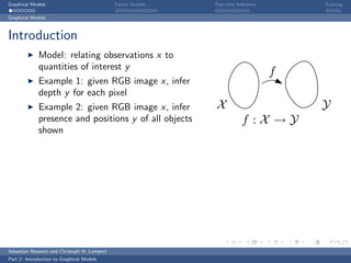
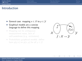
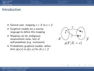
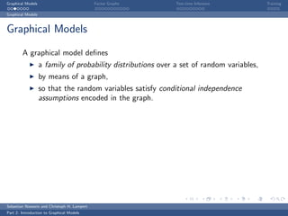
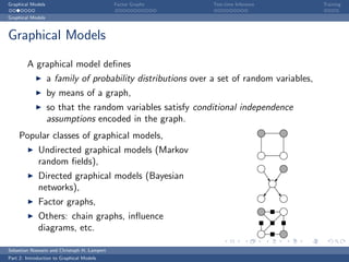
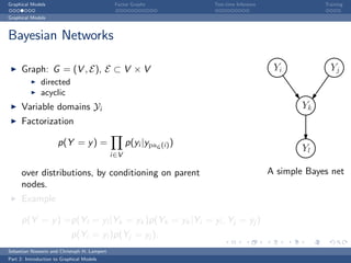
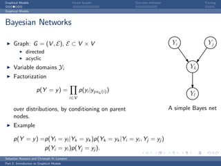
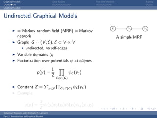
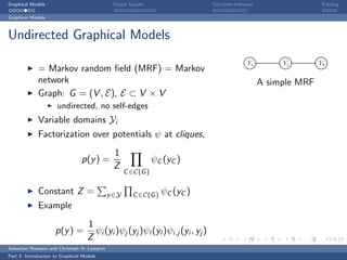
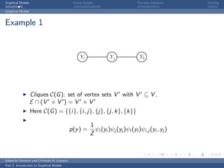
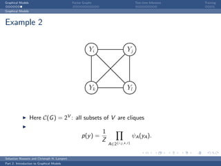
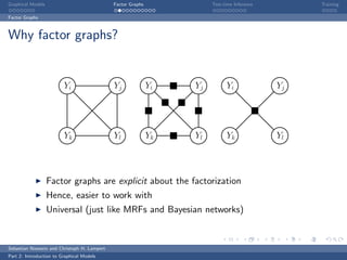
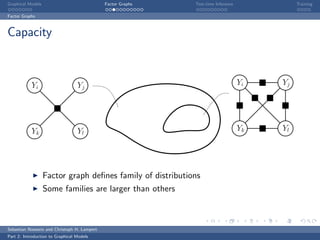
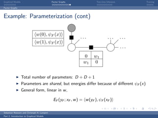
The document is an introduction to graphical models. It discusses that graphical models define probability distributions over random variables using graphs to encode conditional independence assumptions. It then describes popular classes of graphical models including directed Bayesian networks and undirected Markov random fields. Bayesian networks define a factorization of the joint distribution over parent variables, while Markov random fields factorize over potentials at cliques in the graph. An example Markov random field is also shown.


![Graphical Models Factor Graphs Test-time Inference Training
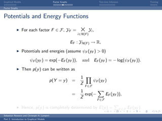
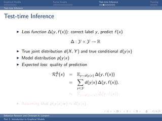
Test-time Inference
Example 2: Hamming loss
Count the number of mislabeled variables:
1
∆H (y , y ∗ ) = I (yi = yi∗ )
|V |
i∈V
Plugging it in,
y∗ := argmin Ey ∼p(y |x) [∆H (y , y )]
y ∈Y
= argmax p(yi |x)
yi ∈Yi
i∈V
Minimizing the expected Hamming loss → maximum posterior
marginal (MPM, Max-Marg) prediction
Sebastian Nowozin and Christoph H. Lampert
Part 2: Introduction to Graphical Models](https://image.slidesharecdn.com/01graphicalmodels-120305024317-phpapp01/85/01-graphical-models-40-320.jpg)
![Graphical Models Factor Graphs Test-time Inference Training
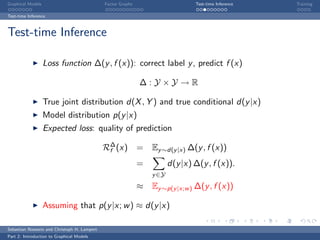
Test-time Inference
Example 2: Hamming loss
Count the number of mislabeled variables:
1
∆H (y , y ∗ ) = I (yi = yi∗ )
|V |
i∈V
Plugging it in,
y∗ := argmin Ey ∼p(y |x) [∆H (y , y )]
y ∈Y
= argmax p(yi |x)
yi ∈Yi
i∈V
Minimizing the expected Hamming loss → maximum posterior
marginal (MPM, Max-Marg) prediction
Sebastian Nowozin and Christoph H. Lampert
Part 2: Introduction to Graphical Models](https://image.slidesharecdn.com/01graphicalmodels-120305024317-phpapp01/85/01-graphical-models-41-320.jpg)
![Graphical Models Factor Graphs Test-time Inference Training
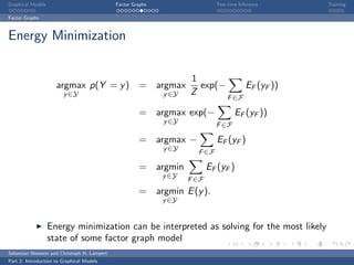
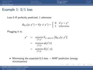
Test-time Inference
Example 3: Squared error
Assume a vector space on Yi (pixel intensities,
optical flow vectors, etc.).
Sum of squared errors
1
∆Q (y , y ∗ ) = yi − yi∗ 2 .
|V |
i∈V
Plugging it in,
y∗ := argmin Ey ∼p(y |x) [∆Q (y , y )]
y ∈Y
= p(yi |x)yi
yi ∈Yi
i∈V
Minimizing the expected squared error → minimum mean squared
error (MMSE) prediction
Sebastian Nowozin and Christoph H. Lampert
Part 2: Introduction to Graphical Models](https://image.slidesharecdn.com/01graphicalmodels-120305024317-phpapp01/85/01-graphical-models-42-320.jpg)
![Graphical Models Factor Graphs Test-time Inference Training
Test-time Inference
Example 3: Squared error
Assume a vector space on Yi (pixel intensities,
optical flow vectors, etc.).
Sum of squared errors
1
∆Q (y , y ∗ ) = yi − yi∗ 2 .
|V |
i∈V
Plugging it in,
y∗ := argmin Ey ∼p(y |x) [∆Q (y , y )]
y ∈Y
= p(yi |x)yi
yi ∈Yi
i∈V
Minimizing the expected squared error → minimum mean squared
error (MMSE) prediction
Sebastian Nowozin and Christoph H. Lampert
Part 2: Introduction to Graphical Models](https://image.slidesharecdn.com/01graphicalmodels-120305024317-phpapp01/85/01-graphical-models-43-320.jpg)
![Graphical Models Factor Graphs Test-time Inference Training
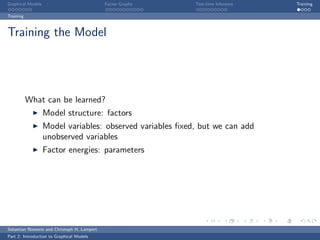
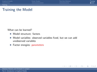
Training
Loss-Minimizing Parameter Learning
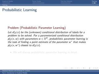
Problem (Loss-Minimizing Parameter Learning)
Let d(x, y ) be the unknown distribution of data in labels, and let
∆ : Y × Y → R be a loss function. Loss minimizing parameter learning is
the task of finding a parameter value w ∗ such that the expected
prediction risk
E(x,y )∼d(x,y ) [∆(y , fp (x))]
is as small as possible, where fp (x) = argmaxy ∈Y p(y |x, w ∗ ).
Requires loss function at training time
Directly learns a prediction function fp (x)
Sebastian Nowozin and Christoph H. Lampert
Part 2: Introduction to Graphical Models](https://image.slidesharecdn.com/01graphicalmodels-120305024317-phpapp01/85/01-graphical-models-53-320.jpg)
![Graphical Models Factor Graphs Test-time Inference Training
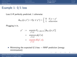
Training
Loss-Minimizing Parameter Learning
Problem (Loss-Minimizing Parameter Learning)
Let d(x, y ) be the unknown distribution of data in labels, and let
∆ : Y × Y → R be a loss function. Loss minimizing parameter learning is
the task of finding a parameter value w ∗ such that the expected
prediction risk
E(x,y )∼d(x,y ) [∆(y , fp (x))]
is as small as possible, where fp (x) = argmaxy ∈Y p(y |x, w ∗ ).
Requires loss function at training time
Directly learns a prediction function fp (x)
Sebastian Nowozin and Christoph H. Lampert
Part 2: Introduction to Graphical Models](https://image.slidesharecdn.com/01graphicalmodels-120305024317-phpapp01/85/01-graphical-models-54-320.jpg)