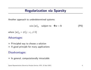
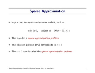
This document summarizes research on sparse representations by Joel Tropp. It discusses how sparse approximation problems arise in applications like variable selection in regression and seismic imaging. It presents algorithms for solving sparse representation problems, including orthogonal matching pursuit and 1-minimization. It analyzes when these algorithms can recover sparse solutions and proves performance guarantees for random matrices and random sparse vectors. The document also discusses related areas like compressive sampling and simultaneous sparsity.

1. Sparse Representations
k
Joel A. Tropp
Department of Mathematics
The University of Michigan
jtropp@umich.edu
Research supported in part by NSF and DARPA 1

2. Introduction
Sparse Representations (Numerical Analysis Seminar, NYU, 20 April 2007) 2

3. Systems of Linear Equations
We consider linear systems of the form
 
 
    
d  Φ   
   

x = b
   
 
 
 
N
Assume that
l Φ has dimensions d × N with N ≥ d
l Φ has full rank
l The columns of Φ have unit 2 norm
Sparse Representations (Numerical Analysis Seminar, NYU, 20 April 2007) 3

4. The Trichotomy Theorem
Theorem 1. For a linear system Φx = b, exactly one of the following
situations obtains.
1. No solution exists.
2. The equation has a unique solution.
3. The solutions form a linear subspace of positive dimension.
Sparse Representations (Numerical Analysis Seminar, NYU, 20 April 2007) 4

5. Minimum-Energy Solutions
Classical approach to underdetermined systems:
min x 2 subject to Φx = b
Advantages:
l Analytically tractable
l Physical interpretation as minimum energy
l Principled way to pick a unique solution
Disadvantages:
l Solution is typically nonzero in every component
l The wrong principle for most applications
Sparse Representations (Numerical Analysis Seminar, NYU, 20 April 2007) 5

6. Regularization via Sparsity
Another approach to underdetermined systems:
min x 0 subject to Φx = b (P0)
where x 0 = #{j : xj = 0}
Advantages:
l Principled way to choose a solution
l A good principle for many applications
Disadvantages:
l In general, computationally intractable
Sparse Representations (Numerical Analysis Seminar, NYU, 20 April 2007) 6

7. Sparse Approximation
l In practice, we solve a noise-aware variant, such as
min x 0 subject to Φx − b 2 ≤ε
l This is called a sparse approximation problem
l The noiseless problem (P0) corresponds to ε = 0
l The ε = 0 case is called the sparse representation problem
Sparse Representations (Numerical Analysis Seminar, NYU, 20 April 2007) 7

8. Applications
Sparse Representations (Numerical Analysis Seminar, NYU, 20 April 2007) 8

9. Variable Selection in Regression
l The oldest application of sparse approximation is linear regression
l The columns of Φ are explanatory variables
l The right-hand side b is the response variable
l Φx is a linear predictor of the response
l Want to use few explanatory variables
l Reduces variance of estimator
l Limits sensitivity to noise
Reference: [Miller 2002]
Sparse Representations (Numerical Analysis Seminar, NYU, 20 April 2007) 9

10. Seismic Imaging
"In deconvolving any observed seismic trace, it is
rather disappointing to discover that there is a
nonzero spike at every point in time regardless of the
data sampling rate. One might hope to find spikes only
where real geologic discontinuities take place."
References: [Claerbout–Muir 1973]
Sparse Representations (Numerical Analysis Seminar, NYU, 20 April 2007) 10

11. Transform Coding
l Transform coding can be viewed as a sparse approximation problem
DCT
−−
−→
IDCT
←−−
−−
Reference: [Daubechies–DeVore–Donoho–Vetterli 1998]
Sparse Representations (Numerical Analysis Seminar, NYU, 20 April 2007) 11

12. Algorithms
Sparse Representations (Numerical Analysis Seminar, NYU, 20 April 2007) 12

13. Sparse Representation is Hard
Theorem 2. [Davis (1994), Natarajan (1995)] Any algorithm that
can solve the sparse representation problem for every matrix and
right-hand side must solve an NP-hard problem.
Sparse Representations (Numerical Analysis Seminar, NYU, 20 April 2007) 13

14. But...
Many interesting instances
of the sparse representation problem
are tractable!
Basic example: Φ is orthogonal
Sparse Representations (Numerical Analysis Seminar, NYU, 20 April 2007) 14

15. Algorithms for Sparse Representation
l Greedy methods make a sequence of locally optimal choices in hope of
determining a globally optimal solution
l Convex relaxation methods replace the combinatorial sparse
approximation problem with a related convex program in hope that the
solutions coincide
l Other approaches include brute force, nonlinear programming, Bayesian
methods, dynamic programming, algebraic techniques...
Refs: [Baraniuk, Barron, Bresler, Cand`s, DeVore, Donoho, Efron, Fuchs,
e
Gilbert, Golub, Hastie, Huo, Indyk, Jones, Mallat, Muthukrishnan, Rao,
Romberg, Stewart, Strauss, Tao, Temlyakov, Tewfik, Tibshirani, Willsky...]
Sparse Representations (Numerical Analysis Seminar, NYU, 20 April 2007) 15

16. Orthogonal Matching Pursuit (OMP)
Input: The matrix Φ, right-hand side b, and sparsity level m
Initialize the residual r0 = b
For t = 1, . . . , m do
A. Find a column most correlated with the residual:
ωt = arg maxj=1,...,N | rt−1, ϕj |
B. Update residual by solving a least-squares problem:
yt = arg miny b − Φt y 2
rt = b − Φt yt
where Φt = [ϕω1 . . . ϕωt ]
Output: Estimate x(ωj ) = ym(j)
Sparse Representations (Numerical Analysis Seminar, NYU, 20 April 2007) 16

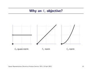
17. 1 Minimization
Sparse Representation as a Combinatorial Problem
min x 0 subject to Φx = b (P0)
Relax to a Convex Program
min x 1 subject to Φx = b (P1)
l Any numerical method can be used to perform the minimization
l Projected gradient and interior-point methods seem to work best
References: [Donoho et al. 1999, Figueredo et al. 2007]
Sparse Representations (Numerical Analysis Seminar, NYU, 20 April 2007) 17

18. Why an 1 objective?
0 quasi-norm 1 norm 2 norm
Sparse Representations (Numerical Analysis Seminar, NYU, 20 April 2007) 18

19. Why an 1 objective?
0 quasi-norm 1 norm 2 norm
Sparse Representations (Numerical Analysis Seminar, NYU, 20 April 2007) 19

20. Relative Merits
OMP (P1)
Computational Cost X
Ease of Implementation X
Effectiveness X
Sparse Representations (Numerical Analysis Seminar, NYU, 20 April 2007) 20

21. When do the
algorithms work?
Sparse Representations (Numerical Analysis Seminar, NYU, 20 April 2007) 21

22. Key Insight
Sparse representation is tractable
when the matrix Φ is sufficiently nice
(More precisely, column submatrices
of the matrix should be well conditioned)
Sparse Representations (Numerical Analysis Seminar, NYU, 20 April 2007) 22

23. Quantifying Niceness
l We say Φ is incoherent when
1
max | ϕj , ϕk | ≤ √
j=k d
l Incoherent matrices appear often in signal processing applications
l We call Φ a tight frame when
N
ΦΦT = I
d
l Tight frames have minimal spectral norm among conformal matrices
Note: Both conditions can be relaxed substantially
Sparse Representations (Numerical Analysis Seminar, NYU, 20 April 2007) 23

24. Example: Identity + Fourier
1
1/√d
Impulses Complex Exponentials
An incoherent tight frame
Sparse Representations (Numerical Analysis Seminar, NYU, 20 April 2007) 24

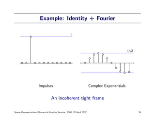
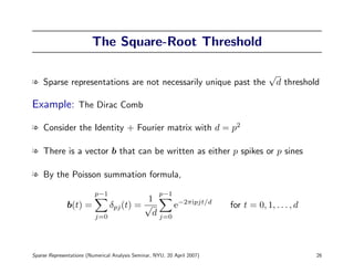
25. Finding Sparse Solutions
Theorem 3. [T 2004] Let Φ be incoherent. Suppose that the linear
system Φx = b has a solution x that satisfies
√
1
x 0 < 2 ( d + 1).
Then the vector x is
1. the unique minimal 0 solution to the linear system, and
2. the output of both OMP and 1 minimization.
References: [Donoho–Huo 2001, Greed is Good, Just Relax]
Sparse Representations (Numerical Analysis Seminar, NYU, 20 April 2007) 25

26. The Square-Root Threshold
√
l Sparse representations are not necessarily unique past the d threshold
Example: The Dirac Comb
l Consider the Identity + Fourier matrix with d = p2
l There is a vector b that can be written as either p spikes or p sines
l By the Poisson summation formula,
p−1 p−1
1
b(t) = δpj (t) = √ e−2πipjt/d for t = 0, 1, . . . , d
j=0
d j=0
Sparse Representations (Numerical Analysis Seminar, NYU, 20 April 2007) 26

27. Enter Probability
Insight:
The bad vectors are atypical
l It is usually possible to identify random sparse vectors
l The next theorem is the first step toward quantifying this intuition
Sparse Representations (Numerical Analysis Seminar, NYU, 20 April 2007) 27

28. Conditioning of Random Submatrices
Theorem 4. [T 2006] Let Φ be an incoherent tight frame with at least
twice as many columns as rows. Suppose that
cd
m ≤ .
log d
If A is a random m-column submatrix of Φ then
1
Prob A∗ A − I < ≥ 99.44%.
2
The number c is a positive absolute constant.
Reference: [Random Subdictionaries]
Sparse Representations (Numerical Analysis Seminar, NYU, 20 April 2007) 28

29. Recovering Random Sparse Vectors
Model (M) for b = Φx
The matrix Φ is an incoherent tight frame
Nonzero entries of x number m ≤ cd/ log N
have uniformly random positions
are independent, zero-mean Gaussian RVs
Theorem 5. [T 2006] Let b = Φx be a random vector drawn according
to Model (M). Then x is
1. the unique minimal 0 solution w.p. at least 99.44% and
2. the unique minimal 1 solution w.p. at least 99.44%.
Reference: [Random Subdictionaries]
Sparse Representations (Numerical Analysis Seminar, NYU, 20 April 2007) 29

30. Methods of Proof
l Functional success criterion for OMP
l Duality results for convex optimization
l Banach algebra techniques for estimating matrix norms
l Concentration of measure inequalities
l Banach space methods for studying spectra of random matrices
l Decoupling of dependent random variables
l Symmetrization of random subset sums
l Noncommutative Khintchine inequalities
l Bounds for suprema of empirical processes
Sparse Representations (Numerical Analysis Seminar, NYU, 20 April 2007) 30

31. Compressive
Sampling
Sparse Representations (Numerical Analysis Seminar, NYU, 20 April 2007) 31

32. Compressive Sampling I
l In many applications, signals of interest have sparse representations
l Traditional methods acquire entire signal, then extract information
l Sparsity can be exploited when acquiring these signals
l Want number of samples proportional to amount of information
l Approach: Introduce randomness in the sampling procedure
l Assumption: Each random sample has unit cost
Sparse Representations (Numerical Analysis Seminar, NYU, 20 April 2007) 32

33. Compressive Sampling II
14.1
–2.6
–5.3
10.4
3.2
sparse signal ( ) linear measurement process data (b = Φx )
l Given data b = Φx, must identify sparse signal x
l This is a sparse representation problem with a random matrix
References: [Cand`s–Romberg–Tao 2004, Donoho 2004]
e
Sparse Representations (Numerical Analysis Seminar, NYU, 20 April 2007) 33

34. Compressive Sampling and OMP
Theorem 6. [T, Gilbert 2005] Assume that
l x is a vector in RN with m nonzeros and
l Φ is a d × N Gaussian matrix with d ≥ Cm log N
l Execute OMP with b = Φx to obtain estimate x
The estimate x equals the vector x with probability at least 99.44%.
Reference: [Signal Recovery via OMP]
Sparse Representations (Numerical Analysis Seminar, NYU, 20 April 2007) 34

35. Compressive Sampling with 1 Minimization
Theorem 7. [Various] Assume that
l Φ is a d × N Gaussian matrix with d ≥ Cm log(N/m)
With probability 99.44%, the following statement holds.
l Let x be a vector in RN with m nonzeros
l Execute 1 minimization with b = Φx to obtain estimate x
The estimate x equals the vector x.
References: [Cand`s et al. 2004–2006], [Donoho et al. 2004–2006],
e
[Rudelson–Vershynin 2006]
Sparse Representations (Numerical Analysis Seminar, NYU, 20 April 2007) 35

36. Related
Directions
Sparse Representations (Numerical Analysis Seminar, NYU, 20 April 2007) 36

37. Sublinear Compressive Sampling
l There are algorithms that can recover sparse signals from random
measurements in time proportional to the number of measurements
l This is an exponential speedup over OMP and 1 minimization
l The cost is a logarithmic number of additional measurements
References: [Algorithmic dimension reduction, One sketch for all]
Joint with Gilbert, Strauss, Vershynin
Sparse Representations (Numerical Analysis Seminar, NYU, 20 April 2007) 37

38. Simultaneous Sparsity
l In some applications, one seeks solutions to the matrix equation
ΦX = B
where X has a minimal number of nonzero rows
l We have studied algorithms for this problem
References: [Simultaneous Sparse Approximation I and II ]
Joint with Gilbert, Strauss
Sparse Representations (Numerical Analysis Seminar, NYU, 20 April 2007) 38

39. Projective Packings
l The coherence statistic plays an important role in sparse representation
l What can we say about matrices Φ with minimal coherence?
l Equivalent to studying packing in projective space
l We have theory about when optimal packings can exist
l We have numerical algorithms for constructing packings
References: [Existence of ETFs, Constructing Structured TFs, . . . ]
Joint with Dhillon, Heath, Sra, Strohmer, Sustik
Sparse Representations (Numerical Analysis Seminar, NYU, 20 April 2007) 39

40. To learn more...
Web: http://www.umich.edu/~jtropp
E-mail: jtropp@umich.edu
Partial List of Papers
l “Greed is good,” Trans. IT, 2004
l “Constructing structured tight frames,” Trans. IT, 2005
l “Just relax,” Trans. IT, 2006
l “Simultaneous sparse approximation I and II,” J. Signal Process., 2006
l “One sketch for all,” to appear, STOC 2007
l “Existence of equiangular tight frames,” submitted, 2004
l “Signal recovery from random measurements via OMP,” submitted, 2005
l “Algorithmic dimension reduction,” submitted, 2006
l “Random subdictionaries,” submitted, 2006
l “Constructing packings in Grassmannian manifolds,” submitted, 2006
Coauthors: Dhillon, Gilbert, Heath, Muthukrishnan, Rice DSP, Sra, Strauss,
Strohmer, Sustik, Vershynin
Sparse Representations (Numerical Analysis Seminar, NYU, 20 April 2007) 40