The document discusses elementary row operations used in solving systems of linear equations, outlining three main types: row exchanges, multiplication by non-zero constants, and addition/subtraction of row multiples. It includes procedures for transforming matrices into upper triangular and unit matrices, as well as determining the inverse of a matrix using the Gauss-Jordan method. Additionally, it covers concepts related to the rank of a matrix, including definitions, methods for calculation, and examples demonstrating these operations.

1. Class: B.Sc CS.
Subject: Discrete Mathematics
Unit-4
RAI UNIVERSITY, AHMEDABAD

2. UNIT-IV-RAW OPERATIONS OF MATRIX
 Elementary Transformations:
 We used the elementary raw operations when we solved system of linear
equations. We'll study them more formally now, and associate each one with
a particular invertible matrix.
 There are three types of Elementary row operations are those operations on
a matrix that don’t change the solution set of the corresponding set of linear
equations.
 Any one of the following operations on a matrix is called an elementary
transformation.
1. Exchange two rows:
Interchange any two rows (or columns). This transformation is indicated
by𝑅𝑖𝑗, if 𝑖𝑡ℎ and 𝑗𝑡ℎ rows are interchanged.
2. Multiply or divide a row by a nonzero constant:
Multiplication of the elements of any row 𝑅𝑖 (or column) by a non zero
Scalar quantity 𝑘 is denoted by 𝑘. 𝑅𝑖
3. Add or subtract a multiple of one row from another:
Addition of constant multiplication of the elements of any row 𝑅𝑗 to the
corresponding elements of any row 𝑅𝑗 to the corresponding elements of
any other row 𝑅𝑗 is denoted by (𝑅𝑖 + 𝑘𝑅𝑗).
Note :
If a matrix B is obtained from a matrix 𝐴 by one or more E-operations, then
B is said to be equivalent to A. The symbol ~ is used for equivalence.
i.e. 𝐴~𝐵
 Example-1. Reduced the following matrix to upper triangular form.
[
1 2 3
2 5 7
3 1 2
]

3. Solution: If in a square matrix , all the elements below the principal
diagonal are zero, the matrix is called an upper triangular matrix.
 [
1 2 3
2 5 7
3 1 2
]
 ~ [
1 2 3
0 1 1
0 −5 −7
] 𝑅2 → 𝑅2 − 2𝑅1 , 𝑅3 → 𝑅3 − 3𝑅1
 ~ [
1 2 3
0 1 1
0 0 −2
] 𝑅3 → 𝑅3 + 5𝑅2
 [
1 2 3
0 1 1
0 0 −2
] is an upper triangular matrix.
 Example-2. Transform [
1 3 3
2 4 10
3 8 4
] in to a unit matrix.
Solution: [
1 3 3
2 4 10
3 8 4
]
 ~ [
1 3 3
0 −2 4
0 −1 −5
] 𝑅2 → 𝑅2 − 2𝑅1 , 𝑅3 → 𝑅3 − 3𝑅1
 ~ [
1 3 3
0 1 −2
0 −1 −5
] 𝑅2 → −
1
2
𝑅2
 ~ [
1 0 9
0 1 −2
0 0 −7
] 𝑅1 → 𝑅1 − 3𝑅2 , 𝑅3 → 𝑅3 + 𝑅2
 ~ [
1 0 9
0 1 −2
0 0 1
] 𝑅3 → −
1
7
𝑅3
 ~ [
1 0 0
0 1 0
0 0 1
] 𝑅1 − 9𝑅3 , 𝑅2 + 2𝑅3

4.  [
1 0 0
0 1 0
0 0 1
] is a Unit matrix.
 Inverse of a matrix by elementary transformations(Gauss Jordan
method):
 The elementary row transformations which reduce a square matrix 𝐴 to
the unit matrix, when applied to the unit matrix, give the inverse matrix
𝐴−1
.
 Let A be non singular square matrix. Then 𝐴 = 𝐼𝐴.
 Apply suitable Elementary row operations to 𝐴 on the left hand side so
that 𝐴 is reduced to 𝐼.
 Simultaneously, apply the same Elementary row operations to the pre-
factor I on right hand side. Let I reduce to 𝐵, so that 𝐼 = 𝐵𝐴.
 Post multiplied by 𝐴−1
, we get
𝐼𝐴−1
= 𝐵𝐴𝐴−1
⟹ 𝐴−1
= 𝐵(𝐴𝐴−1) = 𝐵𝐼 = 𝐵
∴ 𝐵 = 𝐴−1
 Example-1. Find the inverse of the following matrix by using elementary
transformation [
𝟑 −𝟑 𝟒
𝟐 −𝟑 𝟒
𝟎 −𝟏 𝟏
].
Solution: The given matrix is 𝐴 = [
3 −3 4
2 −3 4
0 −1 1
]
 ⟹ [
3 −3 4
2 −3 4
0 −1 1
] = [
1 0 0
0 1 0
0 0 1
] 𝐴
 ⟹ [
1 −1
4
3
2 −3 4
0 −1 1
] = [
1
3
0 0
0 1 0
0 0 1
] 𝐴 𝑅1 →
𝑅1
3

5.  ⟹ [
1 −1
4
3
0 −1
4
3
0 −1 1
] = [
1
3
0 0
−
2
3
1 0
0 0 1
] 𝐴 𝑅2 → 𝑅2 − 2𝑅1
 ⟹ [
1 −1
4
3
0 1 −
4
3
0 −1 1
] = [
1
3
0 0
2
3
−1 0
0 0 1
] 𝐴 𝑅2 → −𝑅2
 ⟹
[
1 −1
4
3
0 1 −
4
3
0 0 −
1
3]
=
[
1
3
0 0
2
3
−1 0
2
3
−1 1]
𝐴 𝑅3 → 𝑅3 + 𝑅2
 ⟹ [
1 −1
4
3
0 1 −
4
3
0 0 1
] = [
1
3
0 0
2
3
−1 0
−2 3 −3
] 𝐴 𝑅3 → −3𝑅3
 [
1 −1 0
0 1 0
0 0 1
] = [
3 −4 4
−2 3 −4
−2 3 −3
] 𝐴 𝑅1 → 𝑅1 −
4
3
𝑅3 , 𝑅2 → 𝑅2 +
4
3
𝑅3
 ⟹ [
1 0 0
0 1 0
0 0 1
] = [
1 −1 0
−2 3 −4
−2 3 −3
] 𝐴 𝑅1 → 𝑅1 + 𝑅2
 Hence 𝐴−1
= [
1 −1 0
−2 3 −4
−3 3 −3
]
 Example-1.find the inverse of 𝑨 = [
𝟎 𝟏 𝟐
𝟏 𝟐 𝟑
𝟑 𝟏 𝟏
] by elementary row
operations.
Solution: The given matrix A is [
0 1 2
1 2 3
3 1 1
]
 ⇒ [
0 1 2
1 2 3
3 1 1
] = [
1 0 0
0 1 0
0 0 1
] 𝐴

6.  ⇒ [
1 2 3
0 1 2
3 1 1
] = [
0 1 0
1 0 0
0 0 1
] 𝑅1 ↔ 𝑅2
 ⇒ [
1 2 3
0 1 2
0 −5 −8
] = [
0 1 0
1 0 0
0 −3 1
] 𝐴 𝑅3 → 𝑅3 − 3𝑅1
 ⇒ [
1 0 −1
0 1 2
0 0 2
] = [
−2 1 0
1 0 0
5 −3 1
] 𝐴 𝑅1 → 𝑅1 − 2𝑅2, 𝑅3 → 𝑅3 + 5𝑅2
 ⇒ [
1 0 −1
0 1 2
0 0 1
] = [
−2 1 0
1 0 0
5
2
−
3
2
1
2
] 𝐴 𝑅3 →
1
2
𝑅3
 ⇒ [
1 0 0
0 1 0
0 0 1
]=[
1
2
−
1
2
1
2
−4 3 −1
5
2
−
3
2
1
2
] 𝐴 𝑅1 → 𝑅1 + 𝑅3, 𝑅2 → 𝑅2 − 2𝑅3
 ⇒ Hence 𝐴−1
= [
1
2
−
1
2
1
2
−4 3 −1
5
2
−
3
2
1
2
]
 Rank Of Matrix:
Let 𝐴 be 𝑚 × 𝑛 matrix. It has square sub-matrices of different orders. The
determinants of these square sub-matrices are called minors of 𝐴. If all
minors of order (𝑟 + 1) are zero but there is at least one non-zero minor of
order 𝑟, then 𝑟 is called the rank of 𝐴.
Symbolically, rank of 𝐴 = 𝑟 is written as 𝜌(𝐴) = 𝑟
Note: From the above definition of the rank of a matrix 𝐴, it follows that:
(i) If A is null matrix then 𝜌(𝐴) = 0
(ii) If A is not a null matrix, then 𝜌(𝐴) ≥ 1
(iii)If A is a non-singular 𝑛 × 𝑛 matrix, then 𝜌(𝐴) = 𝑛
(iv) If 𝐼 𝑛 is the 𝑛 × 𝑛 unit matrix, then |𝐼 𝑛| = 1 ≠ 0 ⟹ 𝜌(𝐼 𝑛) = 𝑛

7. (v) If 𝐴 is an 𝑚 × 𝑛 matrix, then 𝜌(𝐴) ≤ minimum of 𝑚 and 𝑛.
(vi) If all minors of order 𝑟 are equal to zero, then 𝜌(𝐴) < 𝑟.
There are three method for finding Rank of matrix:
1. Determinant Method
2. Triangular form
3. Normal form (canonical form or row reduced echelon form)
1. Determinant Method:
The rank of a matrix is said to be 𝑟 if
(a) It has at least one non-zero minor of order 𝑟.
(b) Every minor of 𝐴 of order higher than 𝑟 is Zero.
Steps for calculate rank by determinant method:
 Step-1: Starts with the highest order minor of 𝐴. Let their order be 𝑟. If any
one of them is non-zero, then 𝜌(𝐴) < 𝑟.
 Step-2: If all of them are zero, start with minors of next lower order (𝑟 − 1)
and so on till you get a non-zero minor. The order of that minor is the rank
of 𝐴.
Note: This method usually involves a lot of computational work since we
have to evaluate several determinants.
 Example-1. Find the rank of the matrix using determinant method.
𝑨 = [
𝟐 𝟓 𝟓
−𝟏 −𝟏 𝟎
𝟐 𝟒 𝟑
]
Solution: |𝐴| = |
2 5 5
−1 −1 0
2 4 3
|
 |𝐴| = 2(−3 − 0) − 5(−3 − 0) + 5(−4 + 2)
 |𝐴| = −6 + 15 − 10
 |𝐴| = −16 + 15

8.  |𝐴| = −1 ≠ 0
 ∴ 𝑟(𝐴) = 3
 𝑖. 𝑒. rank of 𝐴 = 𝑟 = 3
 Example-2. Find the rank of the matrix using determinant method.
𝑨 = [
𝟏 𝟐 𝟑
𝟐 𝟒 𝟔
𝟑 𝟔 𝟗
]
Solution: |𝐴| = |
1 2 3
2 4 6
3 6 9
|
|𝐴| = 1(36 − 36) − 2(18 − 18) + 3(12 − 12)
|𝐴| = 1(0) − 2(0) + 3(0)
|𝐴| = 0
 ∴ 𝑟(𝐴) < 3
 |𝐴1| = |
1 2
2 4
| = 4 − 4 = 0
 |𝐴2| = |
2 3
4 6
| = 12 − 12 = 0
 |𝐴3| = |
1 3
2 6
| = 6 − 6 = 0
 |𝐴4| = |
2 4
3 6
| = 12 − 12 = 0
 |𝐴5| = |
4 6
6 9
| = 36 − 36 = 0
 |𝐴6| = |
2 6
3 9
| = 18 − 18 = 0
 |𝐴7| = |
1 2
3 6
| = 6 − 6 = 0

9.  |𝐴8| = |
2 3
6 9
| = 18 − 18 = 0
 |𝐴9| = |
1 3
3 9
| = 9 − 9 = 0
 Here, all minors are Zeros.
 ∴ 𝑟(𝐴) < 2
 Now, |𝐴11| = 1 ≠ 0
 ∴ 𝑟(𝐴) = 1
 𝑖. 𝑒. rank of 𝐴 = 𝑟 = 1
2. Rank of matrix by Triangular form
Definition: Rank = number of non-zero row in upper triangular matrix.
In this method first of all we convert the matrix in to the triangular form by
using elementary transformation.
 Example-1. Find the rank of the matrix by using triangular form.
[
𝟏 𝟐
𝟐 𝟑
𝟏 𝟑
𝟑 𝟐
𝟓 𝟏
𝟒 𝟓
]
Solution:
 𝐴 = [
1 2
2 3
1 3
3 2
5 1
4 5
]
 ~ [
1 2
0 −1
0 1
3 2
−1 3
1 3
] (−2)𝑅1 + 𝑅2, (−1)𝑅1 + 𝑅3
 ~ [
1 2
0 −1
0 0
3 2
−1 3
0 0
] 𝑅2 + 𝑅3,
 [
1 2
0 −1
0 0
3 2
−1 3
0 0
] is a triangular matrix. In which

10. No. of non zero rows = 2
 ∴ 𝑟(𝐴) = 𝑟 = 2
 Example-2. Use elementary transformation to reduce the following
matrix 𝑨
to triangular form and hence find the rank of 𝑨.
𝑨 = [
𝟐 𝟑 −𝟏
𝟏 −𝟏 −𝟐
𝟑 𝟏 𝟑
𝟏
−𝟒
−𝟐
𝟔 𝟑 −𝟎 −𝟕
]
Solution: 𝐴 = [
2 3 −1
1 −1 −2
3 1 3
1
−4
−2
6 3 −0 −7
]
 ~ [
1 −1 −2
2 3 −1
3 1 3
−4
1
−2
6 3 −0 −7
] 𝑅1 ←→ 𝑅2
 ~ [
1 −1 −2
0 5 3
0 4 9
−4
9
10
0 9 12 17
] 𝑅2 → 𝑅2 − 2𝑅1, 𝑅3 → 𝑅3 − 3𝑅1, 𝑅4 − 6𝑅1
 ~
[
1 −1 −2
0 5 3
0 0
33
5
−4
9
14
5
0 0
33
5
4
5 ]
𝑅3 → 𝑅3 −
4
5
𝑅2, 𝑅4 → 𝑅4 −
9
5
𝑅2
 ~
[
1 −1 −2
0 5 3
0 0
33
5
−4
9
14
5
0 0 0 −
10
5 ]
𝑅4 → 𝑅4 − 𝑅3

11. 
[
1 −1 −2
0 5 3
0 0
33
5
−4
9
14
5
0 0 0 −
10
5 ]
is a triangular matrix in which
No. of non zero rows =4
 ∴ 𝑟(𝐴) = 𝑟 = 4
3. Normal form (Canonical form):
If 𝐴 is 𝑚 × 𝑛 matrix and by a series of elementary transformations, 𝐴 can be
reduced to one of the following forms, called the normal form or canonical
form of 𝐴.
(i) [𝐼𝑟]
(ii)[𝐼𝑟 ∶ 0]
(iii) [
𝐼𝑟
…
0
]
(iv) [
𝐼𝑟 : 0
… … : … …
0 : 0
]
Where 𝐼𝑟 is the unit matrix of order 𝑟,The number of 𝑟 so obtained is
called the rank of 𝐴.
 Example-1. Find the rank of the following matrix by reducing it to
normal or canonical form.
𝑨 = [
𝟏 𝟐 𝟑
𝟐 𝟒 𝟔
𝟑 𝟔 𝟗
]
Solution:
Since 𝐴 = [
1 2 3
2 4 6
3 6 9
]

12. ~ [
1 2 3
0 0 0
0 0 0
] (−2)𝑅1 + 𝑅2 , (−3)𝑅1 + 𝑅3
~ [
1 0 0
0 0 0
0 0 0
] (−2)𝐶1 + 𝐶2, (−3)𝐶1 + 𝐶3
~ [
𝐼1 : 0
… … : … …
0 : 0
]
 Here 𝐼𝑟 = 𝐼1 hence 𝑟 = 1
∴ 𝜌(𝐴) = 𝑟 = 1
 Example-2: Find the rank of the matrix reducing it to normal form
𝑨 = [
−𝟏 𝟐 −𝟐
𝟏 𝟐 𝟏
−𝟏 −𝟏 𝟐
]
Solution:
We have 𝐴 = [
−1 2 −2
1 2 1
−1 −1 2
]
 ~ [
−1 2 −2
0 4 −1
0 −3 4
] 𝑅2 → 𝑅2 + 𝑅1, 𝑅3 → 𝑅3 − 𝑅1
 ~ [
−1 2 −2
0 4 −1
0 0
13
4
] 𝑅3 → 𝑅3 +
3
4
𝑅2
 ~ [
−1 2 −2
0 4 −1
0 0 1
] 𝑅3 →
4
13
𝑅3
 ~ [
−1 2 0
0 4 0
0 0 1
] 𝑅1 → 𝑅1 + 2𝑅3, 𝑅2 → 𝑅2 + 𝑅3
 ~ [
−1 2 0
0 1 0
0 0 1
] 𝑅2 →
1
4
𝑅2

13.  ~ [
−1 0 0
0 1 0
0 0 1
] 𝑅1 → 𝑅1 − 2𝑅2
 ~ [
1 0 0
0 1 0
0 0 1
] 𝑅1 → (−1)𝑅1
 [
1 0 0
0 1 0
0 0 1
] = [𝐼3] = [𝐼𝑟]
 ∴ 𝑟 = 3
 ℎ𝑒𝑛𝑐𝑒 𝜌(𝐴) = 𝑟 = 3
 Example-3. Reduce the matrix to normal form and find its rank.
𝑨 = [
𝟐 𝟑 𝟒 𝟓
𝟑 𝟒 𝟓
𝟒 𝟓 𝟔
𝟗 𝟏𝟎 𝟏𝟏
𝟔
𝟕
𝟏𝟐
]
Solution: We have
𝐴 = [
2 3 4 5
3 4 5
4 5 6
9 10 11
6
7
12
]
 ~𝐴 =
[
2 3 4 5
0 −
1
2
−1
0 −1 −2
0 −
7
2
−7
−
3
2
−3
−
21
2 ]
𝑅2 → 𝑅2 −
3
2
𝑅1, 𝑅3 → 𝑅3 − 2𝑅1, 𝑅4 → 𝑅4 −
9
2
𝑅1

14.  ~𝐴 =
[
2 0 0 0
0 −
1
2
−1
0 −1 −2
0 −
7
2
−7
−
3
2
−3
−
21
2 ]
𝐶2 → 𝐶2 −
3
2
𝐶1, 𝐶3 → 𝐶3 − 2𝐶1, 𝐶4 → 𝐶4 −
9
2
𝐶1
 ~𝐴 = [
1 0 0 0
0 1 2
0 1 2
0 1 2
3
3
3
]
𝑅1 →
1
2
𝑅1, 𝑅2 → −2𝑅2, 𝑅3 → −𝑅3 , 𝑅4 → −
2
7
𝑅4
 ~𝐴 = [
1 0 0 0
0 1 2
0 0 0
0 0 0
3
0
0
] 𝑅3 → 𝑅3 − 𝑅2, 𝑅4 → 𝑅4 − 𝑅2
 ~𝐴 = [
1 0 0 0
0 1 0
0 0 0
0 0 0
0
0
0
] 𝐶3 → 𝐶3 − 2𝐶2, 𝐶4 → 𝐶4 − 3𝐶2
 ~𝐴 = [
𝐼2 0 0
0 0 0
0 0 0
] = [
𝐼𝑟 : 0
… … : … …
0 : 0
]
 ∴ 𝐼𝑟 = 𝐼2
 ∴ 𝜌(𝐴) = 𝑟 = 2
 Row echelon form and Reduced Row echelon form:
Rules:
1. If the row does not consist entirely zeros then the first non-zero
number in the row is 1.This 1 is called ‘leading 1’
2. If there are any rows that consist entirely of zeros, then they are
grouped together at the bottom of the matrix.

15. 3. If any two successive rows that do not consist entirely of zeros,the
leading 1 in the lower row occurs further to the right than the leading
1 in higher row.
4. Each column that contains a leading 1 has zeros everywhere else in
that column.
A matrix having first three properties is called to be in row echelon form.
A matrix having all four properties is said to be in reduced row echelon
form
Example for,
 [
1 4 −3
0 1 6
0 0 1
7
3
−5
] Row echelon form
 [
1 0 0
0 1 0
0 0 1
0
0
0
] Reduced Row echelon form
 [
0 0 0
0 0 0
0 0 0
] Row echelon & Reduced Row echelon form
 [
0 1 0
0 0 0
1 0 0
] neither Row echelon & Reduced Row echelon form
 [
1 2 3
0 0 1
0 0 0
] Row echelon form
 [
1 0 0
0 1 0
0 0 1
5
3
7
] Reduced Row echelon form
 [
1 2 0
0 0 1
0 0 0
5
7
0
] Reduced Row echelon form

16.  Example-1 Reduced the following matrices to Reduced Row Echelon
form. [
𝟏 𝟐 𝟏
−𝟐 −𝟑 𝟏
𝟑 𝟓 𝟎
]
Solution:
 Given matrix 𝐴 = [
1 2 1
−2 −3 1
3 5 0
]
 ~ [
1 2 1
0 1 3
3 5 0
] 𝑅2 → 2𝑅1 + 𝑅2,
 ~ [
1 2 1
0 1 3
0 −1 −3
] 𝑅3 → (−3)𝑅1 + 𝑅3
 ~ [
1 2 1
0 1 3
0 0 0
] 𝑅3 → 𝑅2 + 𝑅3
 We are now in row echelon form. So we continue proceeding for Reduced
row echelon form
 ~ [
1 0 −5
0 1 3
0 0 0
] 𝑅2 → (−2)𝑅2 + 𝑅1
 The matrix is now in Reduced Row echelon form.
Note:
A matrix is in Reduced Row Echelon Form provided:
 The first non zero entry in any row is the number 1, these are called pivots.
(So each row can have zero or one pivot)
 A pivot is the only non-zero entry in its column. (So each column can have
zero or one pivot)
 Rows are orders so that rows of all zeros are at the bottom and the pivots are
in column order.

17. Examples of matrix which are not in reduced row echelon form:
 [
1 0 5
0 1 3
0 0 1
] Fails rule -2
 [
1 0 5
0 2 1
0 0 0
] Fails rule-1
 [
0 1 0
1 0 0
0 0 1
] Fails rule -3
 [
0 0 0
1 0 0
0 0 1
] Fails rule-3
 Inverse of the matrix by Reduced Row Echelon form:
 Example-1. Find the Inverse of the following matrix by using Reduced
Row Echelon form:
[
𝟎 𝟏 𝟐
𝟏 𝟐 𝟑
𝟑 𝟏 𝟏
]
Solution:
Solution: The given matrix A is [
0 1 2
1 2 3
3 1 1
]
 ⇒ [
0 1 2
1 2 3
3 1 1
] = [
1 0 0
0 1 0
0 0 1
] 𝐴
 ⇒ [
1 2 3
0 1 2
3 1 1
] = [
0 1 0
1 0 0
0 0 1
] 𝑅1 ↔ 𝑅2
 ⇒ [
1 2 3
0 1 2
0 −5 −8
] = [
0 1 0
1 0 0
0 −3 1
] 𝐴 𝑅3 → 𝑅3 − 3𝑅1
 ⇒ [
1 0 −1
0 1 2
0 0 2
] = [
−2 1 0
1 0 0
5 −3 1
] 𝐴 𝑅1 → 𝑅1 − 2𝑅2, 𝑅3 → 𝑅3 + 5𝑅2
 ⇒ [
1 0 −1
0 1 2
0 0 1
] = [
−2 1 0
1 0 0
5
2
−
3
2
1
2
] 𝐴 𝑅3 →
1
2
𝑅3

18.  ⇒ [
1 0 0
0 1 0
0 0 1
]=[
1
2
−
1
2
1
2
−4 3 −1
5
2
−
3
2
1
2
] 𝐴 𝑅1 → 𝑅1 + 𝑅3, 𝑅2 → 𝑅2 − 2𝑅3
 ⇒ Hence 𝐴−1
= [
1
2
−
1
2
1
2
−4 3 −1
5
2
−
3
2
1
2
]
 Linear dependence and Independence of Vectors:
Vectors (matrices) 𝑋1, 𝑋2,𝑋3,…..𝑋 𝑛 are said to be dependent if
i. All the vectors are of the same order.
ii. n scalars 𝜆1, 𝜆2, 𝜆3, … … … . 𝜆 𝑛, (not all zero) exist such that
𝜆1 𝑋1 + 𝜆2 𝑋2 + 𝜆3 𝑋3 + ⋯ … … + 𝜆 𝑛 𝑋 𝑛=0
Otherwise they are linearly independent.
 Example-1. Check the system of vectors
𝑿 𝟏 = (𝟐, 𝟐, 𝟏) 𝑻
, 𝑿 𝟐 = (𝟏, 𝟑, 𝟏) 𝑻
, 𝑿 𝟑 = (𝟏, 𝟐, 𝟐) 𝑻
are linearly dependent
or not?
Solution:
 Consider the matrix equation
𝜆1 𝑋1 + 𝜆2 𝑋2 + 𝜆3 𝑋3 = 0 ………………………………………..(1)
 𝜆1 [
2
2
1
] + 𝜆2 [
1
3
1
] + 𝜆3 [
1
2
2
] = [
0
0
0
]
2𝜆1 + 𝜆2 + 𝜆3 = 0 ,
2𝜆1 + 3𝜆2 + 2𝜆3 = 0 , and 𝜆1 + 𝜆2 + 2𝜆3 = 0
 [
2 1 1
2 3 2
1 1 2
] [
𝜆1
𝜆2
𝜆3
] = [
0
0
0
]
 [
1 1 2
2 3 2
2 1 1
] [
𝜆1
𝜆2
𝜆3
] = [
0
0
0
] 𝑅1 ↔ 𝑅3

19.  [
1 1 2
0 1 −2
0 −1 −3
] [
𝜆1
𝜆2
𝜆3
] = [
0
0
0
] 𝑅2 → 𝑅2 − 2𝑅1, 𝑅3 → 𝑅3 − 2𝑅1
 [
1 1 2
0 1 −2
0 0 −5
] [
𝜆1
𝜆2
𝜆3
] = [
0
0
0
] 𝑅3 → 𝑅3 + 𝑅2
 𝜆1 + 𝜆2+2𝜆3 = 0
𝜆2 − 2𝜆3 = 0
-5 𝜆3 = 0 ⟹ 𝜆3 = 0
 ∴ 𝜆2 = 0 & 𝜆1 = 0
 Thus non- zero values 𝜆1, 𝜆2, 𝜆3 do not exist which can satisfy (1).
 Hence by definition, the given system of vectors is not linearly dependent.
 Example-2. Examine the following vectors are linear dependent or not?
𝑿 𝟏 = (𝟏, 𝟐, 𝟒), 𝑿 𝟐 = (𝟐, −𝟏, 𝟑), 𝑿 𝟑 = (𝟎, 𝟏, 𝟐), 𝑿 𝟒 = (−𝟑, 𝟕, 𝟐)
Solution:
 Consider the matrix equation
𝜆1 𝑋1 + 𝜆2 𝑋2 + 𝜆3 𝑋3 + 𝜆4 𝑋4 = 0
 𝜆1(1,2,4) + 𝜆2(2, −1,3) + 𝜆3(0,1,2) + 𝜆4(−3,7,2) = 0
 𝜆1 + 2𝜆2 + 0𝜆3 − 3𝜆4 = 0
2𝜆1 − 𝜆2 + 𝜆3 + 7𝜆4 = 0
4𝜆1 + 3𝜆2 + 2𝜆3 + 2𝜆4 = 0
 This is the homogeneous system
[
1 2 0
2 −1 1
4 3 2
−3
7
2
] [
𝜆1
𝜆2
𝜆3
𝜆4
] = [
0
0
0
]
 [
1 2 0
0 −5 1
0 −5 2
−3
13
14
] [
𝜆1
𝜆2
𝜆3
𝜆4
] = [
0
0
0
] 𝑅2 → 𝑅2 − 2𝑅1, 𝑅3 → 𝑅3 − 4𝑅1
 [
1 2 0
0 −5 1
0 −5 2
−3
13
14
] [
𝜆1
𝜆2
𝜆3
𝜆4
] = [
0
0
0
] 𝑅3 → 𝑅3 − 𝑅2

20.  𝜆1 + 2𝜆2 − 3𝜆4 = 0
−5𝜆2 + 𝜆3 + 13𝜆4 = 0
𝜆3 + 𝜆4 = 0
 Let 𝜆4 = 𝑡 ⟹ 𝜆3 + 𝑡 = 0, ⟹ 𝜆3 = −𝑡
 −5𝜆2 − 𝑡 + 13𝑡 = 0 ⟹ 𝜆2 =
12𝑡
5
 𝜆1 +
24𝑡
5
− 3𝑡 = 0 ⟹ 𝜆1 = −
9𝑡
5
 Hence 𝜆1 𝑋1 + 𝜆2 𝑋2 + 𝜆3 𝑋3 + 𝜆4 𝑋4 = 0
But 𝜆1 ≠ 0, 𝜆2 ≠ 0, , 𝜆3 ≠ 0, 𝜆4 ≠ 0
 ∴ The given vectors are linearly dependent.
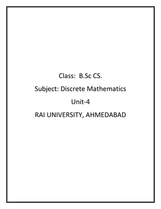
 Linear Dependence and Independence of vector by rank method:
1. If the rank of the matrix of the given vectors is equal to number of vectors
then the vectors are linearly independent.
2. If the rank of the matrix of the given vectors is less than the number of
vectors, then the vectors are linearly dependent.
 Example-1. Show using a matrix that the set of vectors 𝑿 = [𝟏, 𝟐, −𝟑, 𝟒],
𝒀 = [𝟑, −𝟏, 𝟐, 𝟏], 𝒁 = [𝟏, −𝟓, 𝟖, −𝟕] is linearly dependent.
Solution: Here, we have
 𝑋 = [1,2, −3,4], 𝑌 = [3, −1,2,1], 𝑍 = [1, −5,8, −7]
 Let us from a matrix of the above vectors
[
1 2 −3
3 −1 2
1 −5 8
4
1
−7
]
 ~ [
1 2 −3
0 −7 11
0 −7 11
4
−11
−11
] 𝑅2 → 𝑅2 − 3𝑅1, 𝑅3 → 𝑅3 − 𝑅1
 ~ [
1 2 −3
0 −7 11
0 0 0
4
−11
0
] 𝑅3 → 𝑅3 − 𝑅2
 [
1 2 −3
0 −7 11
0 0 0
4
−11
0
] is a triangular matrix in which
 No. of non zero rows = 2 ∴ 𝑟𝑎𝑛𝑘 = 𝑟 = 2
 No. of vectors =3

21.  ∴ the rank of the matrix = 2 < No. of vectors =3
 Hence, vectors are linearly dependent.
 Reference Book and Website Name:
1. Introduction to Engineering Mathematics-1 by H.K. Dass and Dr.Rama
Verma. (S.Chand)
2. A Textbook of Engineering mathematics by N.P.Bali and Dr.Manish
goyal
3. http://aleph0.clarku.edu/~djoyce/ma130/elementary.pdf
4. http://www.math.fsu.edu/~bellenot/class/f08/lalab/other/rref2.pdf

22. EXERCISE-4
Q-1. Evaluate the following questions:
1. Reduce the following matrix to triangular form:
[
1 2 3
2 5 7
3 1 2
]
2. Reduce the following matrix to Identity Matrix:
[
3 1 4
1 2 −5
0 1 5
]
3. Find the inverse of the matrix by using gauss Jordan method
[
1 −1 1
4 1 0
8 1 1
]
4. Find the inverse of the matrix by using gauss Jordan method
[
1 3 3
1 4 3
1 3 4
]
Q.2. Find the rank of following matrices:
1. [
1 2 1
−1 0 2
2 1 −3
]
2. [
0 1 2
4 0 2
2 1 3
−2
6
1
]
3. [
3 2 5
1 1 2
3 3 6
7 12
3 5
9 15
]
4. [
1 2 3
2 4 6
3 6 9
]

23. Q.3. Evaluate the following Questions:
1. Reduced the following matrices to Reduced Row Echelon form.
[
1 3 3
2 4 10
3 8 4
]
2. Reduced the following matrices to Row Echelon form.
[
3 −4 −5
−9 1 4
−5 3 1
]
3. Examine that following system of vectors are linear dependence or not.
[1,0,2,1], [3,1,2,1], [4,6,2, −4], [−6,0, −3, −4]
4. Examine that following system of vectors are linear independence or not.
[1,2, −2] 𝑇
, [−1,3,0] 𝑇
, [−2,0,1] 𝑇